文章目录
1、前言
1.1、定义
- 聚类分析,即聚类,是一项无监督的机器学习任务。它包括自动发现数据中的自然分组。与监督学习(类似预测建模)不同,聚类算法只解释输入数据,并在特征空间中找到自然组或群集。
1.2、数据
- 我们将使用 make _ classification ()函数创建一个测试二分类数据集。数据集将有1000个示例,每个类有两个输入要素和一个群集。这些群集在两个维度上是可见的,因此我们可以用散点图绘制数据,并通过指定的群集对图中的点进行颜色绘制。
# 综合分类数据集
import numpy as np
from sklearn.datasets import make_classification
import matplotlib.pyplot as plt
# 定义数据集
X, y = make_classification(n_samples=1000, n_features=2, n_informative=2, n_redundant=0, n_clusters_per_class=1, random_state=4)
# 为每个类的样本创建散点图
for class_value in range(2):
# 获取此类的示例的行索引
    row_ix = np.where(y == class_value)
    # 创建这些样本的散布
    plt.scatter(X[row_ix, 0], X[row_ix, 1])
    # 绘制散点图
plt.show()
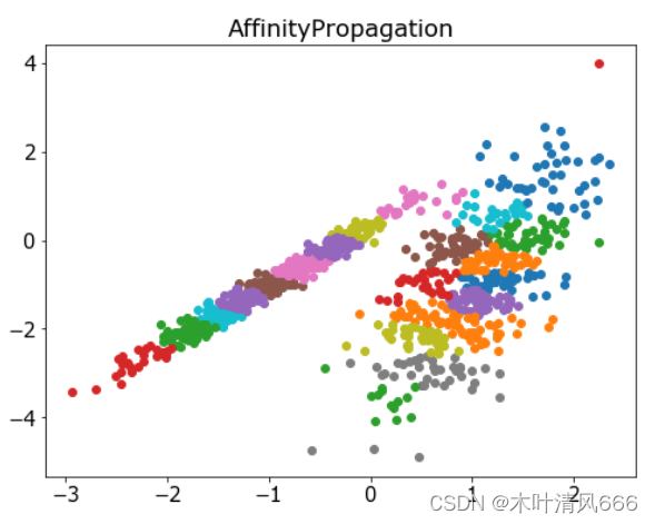
2、亲和力传播
- 它是通过 AffinityPropagation 类实现的,要调整的主要配置是将“ 阻尼 ”设置为0.5到1,甚至可能是“首选项”。
# 亲和力传播聚类 import numpy as np import matplotlib.pyplot as plt from sklearn.datasets import make_classification from sklearn.cluster import AffinityPropagation # 定义数据集 X, _ = make_classification(n_samples=1000, n_features=2, n_informative=2, n_redundant=0, n_clusters_per_class=1, random_state=4) # 定义模型 model = AffinityPropagation(damping=0.9) # 匹配模型 model.fit(X) # 为每个示例分配一个集群 yhat = model.predict(X) # 检索唯一群集 clusters = np.unique(yhat) # 为每个群集的样本创建散点图 plt.figure(figsize=(8,6)) plt.rcParams['font.size']=15 for cluster in clusters: # 获取此群集的示例的行索引 row_ix = np.where(yhat == cluster) # 创建这些样本的散布 plt.scatter(X[row_ix, 0], X[row_ix, 1]) plt.title('AffinityPropagation') # 绘制散点图 plt.show() - 结果
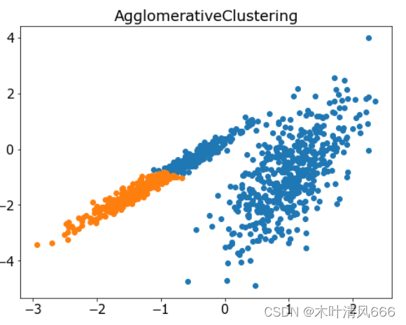
3、聚合聚类
- 聚合聚类涉及合并示例,直到达到所需的群集数量为止。它是层次聚类方法的更广泛类的一部分,通过 AgglomerationClustering 类实现的,主要配置是“ n _ clusters ”集,这是对数据中的群集数量的估计。
# 聚合聚类 import numpy as np import matplotlib.pyplot as plt from sklearn.datasets import make_classification from sklearn.cluster import AgglomerativeClustering # 定义数据集 X, _ = make_classification(n_samples=1000, n_features=2, n_informative=2, n_redundant=0, n_clusters_per_class=1, random_state=4) # 定义模型 model = AgglomerativeClustering(n_clusters=2) # 模型拟合与聚类预测 yhat = model.fit_predict(X) # 检索唯一群集 clusters = np.unique(yhat) # 为每个群集的样本创建散点图 plt.figure(figsize=(8,6)) plt.rcParams['font.size']=15 for cluster in clusters: # 获取此群集的示例的行索引 row_ix = np.where(yhat == cluster) # 创建这些样本的散布 plt.scatter(X[row_ix, 0], X[row_ix, 1]) plt.title('AgglomerativeClustering') # 绘制散点图 plt.show() - 结果
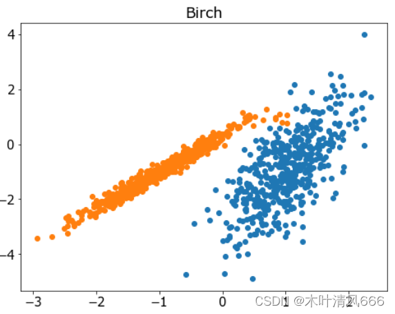
4、BIRCH
- BIRCH 聚类( BIRCH 是平衡迭代减少的缩写,聚类使用层次结构)包括构造一个树状结构,从中提取聚类质心。它是通过 Birch 类实现的,主要配置是“ threshold ”和“ n _ clusters ”超参数,后者提供了群集数量的估计。
# 聚合聚类 import numpy as np import matplotlib.pyplot as plt from sklearn.datasets import make_classification from sklearn.cluster import Birch # 定义数据集 X, _ = make_classification(n_samples=1000, n_features=2, n_informative=2, n_redundant=0, n_clusters_per_class=1, random_state=4) # 定义模型 model = Birch(threshold=0.01, n_clusters=2) # 模型拟合与聚类预测 yhat = model.fit_predict(X) # 检索唯一群集 clusters = np.unique(yhat) # 为每个群集的样本创建散点图 plt.figure(figsize=(8,6)) plt.rcParams['font.size']=15 for cluster in clusters: # 获取此群集的示例的行索引 row_ix = np.where(yhat == cluster) # 创建这些样本的散布 plt.scatter(X[row_ix, 0], X[row_ix, 1]) plt.title('Birch') # 绘制散点图 plt.show() - 结果
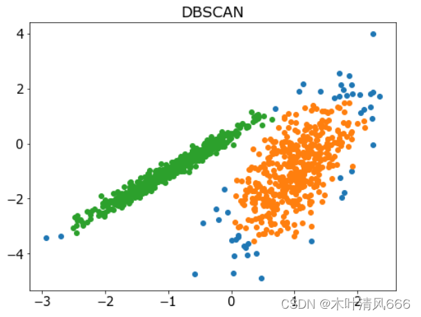
5、DBSCAN
- DBSCAN 聚类(其中 DBSCAN 是基于密度的空间聚类的噪声应用程序)涉及在域中寻找高密度区域,并将其周围的特征空间区域扩展为群集。它是通过 DBSCAN 类实现的,主要配置是“ eps ”和“ min _ samples ”超参数。
# 聚合聚类 import numpy as np import matplotlib.pyplot as plt from sklearn.datasets import make_classification from sklearn.cluster import DBSCAN # 定义数据集 X, _ = make_classification(n_samples=1000, n_features=2, n_informative=2, n_redundant=0, n_clusters_per_class=1, random_state=4) # 定义模型 model = DBSCAN(eps=0.30, min_samples=9) # 模型拟合与聚类预测 yhat = model.fit_predict(X) # 检索唯一群集 clusters = np.unique(yhat) # 为每个群集的样本创建散点图 plt.figure(figsize=(8,6)) plt.rcParams['font.size']=15 for cluster in clusters: # 获取此群集的示例的行索引 row_ix = np.where(yhat == cluster) # 创建这些样本的散布 plt.scatter(X[row_ix, 0], X[row_ix, 1]) plt.title('DBSCAN') # 绘制散点图 plt.show() - 结果
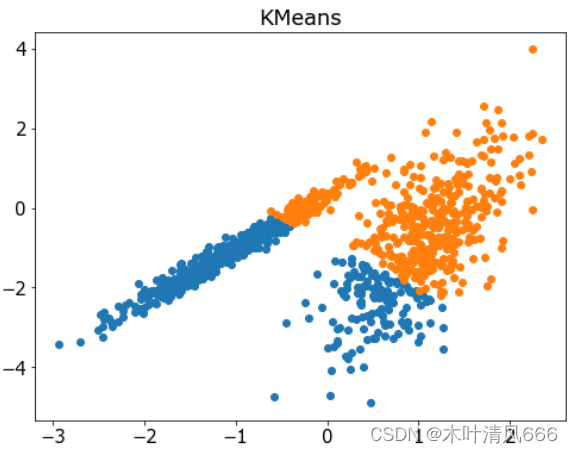
6、K-均值
- K-均值聚类可以是最常见的聚类算法,并涉及向群集分配示例,以尽量减少每个群集内的方差。它是通过 K-均值类实现的,要优化的主要配置是“ n _ clusters ”超参数设置为数据中估计的群集数量。
# 聚合聚类 import numpy as np import matplotlib.pyplot as plt from sklearn.datasets import make_classification from sklearn.cluster import KMeans # 定义数据集 X, _ = make_classification(n_samples=1000, n_features=2, n_informative=2, n_redundant=0, n_clusters_per_class=1, random_state=4) # 定义模型 model = KMeans(n_clusters=2) # 模型拟合与聚类预测 yhat = model.fit_predict(X) # 检索唯一群集 clusters = np.unique(yhat) # 为每个群集的样本创建散点图 plt.figure(figsize=(8,6)) plt.rcParams['font.size']=15 for cluster in clusters: # 获取此群集的示例的行索引 row_ix = np.where(yhat == cluster) # 创建这些样本的散布 plt.scatter(X[row_ix, 0], X[row_ix, 1]) plt.title('KMeans') # 绘制散点图 plt.show() - 结果
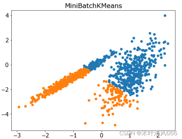
7、Mini-Batch K-均值
- Mini-Batch K-均值是 K-均值的修改版本,它使用小批量的样本而不是整个数据集对群集质心进行更新,这可以使大数据集的更新速度更快,并且可能对统计噪声更健壮。它是通过 MiniBatchKMeans 类实现的,要优化的主配置是“ n _ clusters ”超参数,设置为数据中估计的群集数量。
# 聚合聚类 import numpy as np import matplotlib.pyplot as plt from sklearn.datasets import make_classification from sklearn.cluster import MiniBatchKMeans # 定义数据集 X, _ = make_classification(n_samples=1000, n_features=2, n_informative=2, n_redundant=0, n_clusters_per_class=1, random_state=4) # 定义模型 model = MiniBatchKMeans(n_clusters=2) # 模型拟合与聚类预测 yhat = model.fit_predict(X) # 检索唯一群集 clusters = np.unique(yhat) # 为每个群集的样本创建散点图 plt.figure(figsize=(8,6)) plt.rcParams['font.size']=15 for cluster in clusters: # 获取此群集的示例的行索引 row_ix = np.where(yhat == cluster) # 创建这些样本的散布 plt.scatter(X[row_ix, 0], X[row_ix, 1]) plt.title('MiniBatchKMeans') # 绘制散点图 plt.show() - 结果
8、均值漂移聚类
- 均值漂移聚类涉及到根据特征空间中的实例密度来寻找和调整质心。它是通过 MeanShift 类实现的,主要配置是“带宽”超参数。
# 聚合聚类 import numpy as np import matplotlib.pyplot as plt from sklearn.datasets import make_classification from sklearn.cluster import MeanShift # 定义数据集 X, _ = make_classification(n_samples=1000, n_features=2, n_informative=2, n_redundant=0, n_clusters_per_class=1, random_state=4) # 定义模型 model = MeanShift() # 模型拟合与聚类预测 yhat = model.fit_predict(X) # 检索唯一群集 clusters = np.unique(yhat) # 为每个群集的样本创建散点图 plt.figure(figsize=(8,6)) plt.rcParams['font.size']=15 for cluster in clusters: # 获取此群集的示例的行索引 row_ix = np.where(yhat == cluster) # 创建这些样本的散布 plt.scatter(X[row_ix, 0], X[row_ix, 1]) plt.title('MeanShift') # 绘制散点图 plt.show() - 结果

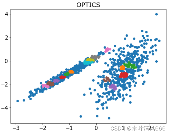
9、OPTICS
- OPTICS 聚类( OPTICS 短于订购点数以标识聚类结构)是上述 DBSCAN 的修改版本。它是通过 OPTICS 类实现的,主要配置是“ eps ”和“ min _ samples ”超参数。
# 聚合聚类 import numpy as np import matplotlib.pyplot as plt from sklearn.datasets import make_classification from sklearn.cluster import OPTICS # 定义数据集 X, _ = make_classification(n_samples=1000, n_features=2, n_informative=2, n_redundant=0, n_clusters_per_class=1, random_state=4) # 定义模型 model = OPTICS(eps=0.8, min_samples=10) # 模型拟合与聚类预测 yhat = model.fit_predict(X) # 检索唯一群集 clusters = np.unique(yhat) # 为每个群集的样本创建散点图 plt.figure(figsize=(8,6)) plt.rcParams['font.size']=15 for cluster in clusters: # 获取此群集的示例的行索引 row_ix = np.where(yhat == cluster) # 创建这些样本的散布 plt.scatter(X[row_ix, 0], X[row_ix, 1]) plt.title('OPTICS') # 绘制散点图 plt.show() - 结果
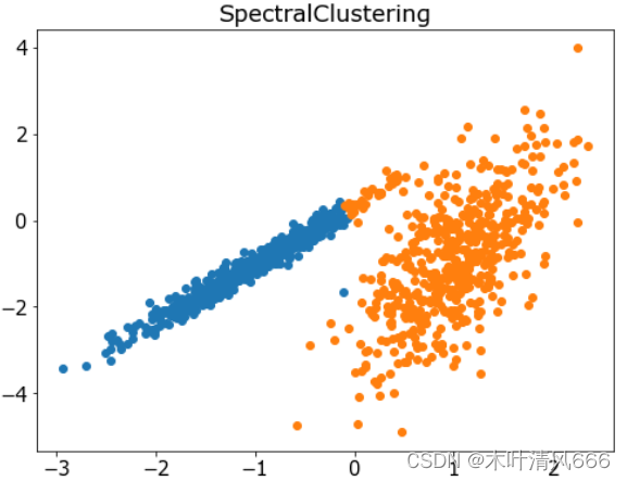
10、光谱聚类
- 光谱聚类是一类通用的聚类方法,取自线性线性代数。它是通过 Spectral 聚类类实现的,而主要的 Spectral 聚类是一个由聚类方法组成的通用类,取自线性线性代数。要优化的是“ n _ clusters ”超参数,用于指定数据中的估计群集数量。
# 聚合聚类 import numpy as np import matplotlib.pyplot as plt from sklearn.datasets import make_classification from sklearn.cluster import SpectralClustering # 定义数据集 X, _ = make_classification(n_samples=1000, n_features=2, n_informative=2, n_redundant=0, n_clusters_per_class=1, random_state=4) # 定义模型 model = SpectralClustering(n_clusters=2) # 模型拟合与聚类预测 yhat = model.fit_predict(X) # 检索唯一群集 clusters = np.unique(yhat) # 为每个群集的样本创建散点图 plt.figure(figsize=(8,6)) plt.rcParams['font.size']=15 for cluster in clusters: # 获取此群集的示例的行索引 row_ix = np.where(yhat == cluster) # 创建这些样本的散布 plt.scatter(X[row_ix, 0], X[row_ix, 1]) plt.title('SpectralClustering') # 绘制散点图 plt.show() - 结果
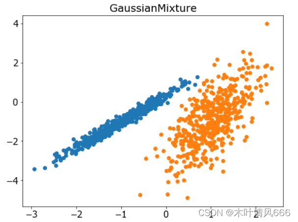
11、高斯混合模型
- 高斯混合模型总结了一个多变量概率密度函数,顾名思义就是混合了高斯概率分布。它是通过 Gaussian Mixture 类实现的,要优化的主要配置是“ n _ clusters ”超参数,用于指定数据中估计的群集数量。
# 聚合聚类 import numpy as np import matplotlib.pyplot as plt from sklearn.datasets import make_classification from sklearn.mixture import GaussianMixture # 定义数据集 X, _ = make_classification(n_samples=1000, n_features=2, n_informative=2, n_redundant=0, n_clusters_per_class=1, random_state=4) # 定义模型 model = GaussianMixture(n_components=2) # 模型拟合与聚类预测 yhat = model.fit_predict(X) # 检索唯一群集 clusters = np.unique(yhat) # 为每个群集的样本创建散点图 plt.figure(figsize=(8,6)) plt.rcParams['font.size']=15 for cluster in clusters: # 获取此群集的示例的行索引 row_ix = np.where(yhat == cluster) # 创建这些样本的散布 plt.scatter(X[row_ix, 0], X[row_ix, 1]) plt.title('GaussianMixture') # 绘制散点图 plt.show() - 结果
12、参考
10 种聚类算法的完整 Python 操作示例


