数据集heart_learning.csv与heart_test.csv是关于心脏病的数据集,heart_learning.csv是训练数据集,heart_test.csv是测试数据集。要求:target和target2为因变量,其他诸变量为自变量。用决策树模型对target和target2做预测,并与实际值比较来验证预测情况。变量说明:pain,ekg,slope,thal是分类变量,在做模型训练前需要对其进行转换为因子型变量。target是定类多值因变量,target2是二值变量,文中分别对其进行预测。
| 变量名称 | 变量说明 |
| age | 年龄 |
| sex | 性别,取值1代表男性,0代表女性 |
| pain | 胸痛的类型,取值1,2,3,4,代表4种类型 |
| bpress | 入院时的静息血压(单位:毫米汞柱) |
| chol | 血清胆固醇(单位:毫克/分升) |
| bsugar | 空腹血糖是否大于120毫克/公升,1代表是,0代表否 |
| ekg | 静息心电图结果,取值0,1,2代表3中不同的结果 |
| thalach | 达到的最大心率 |
| exang | 是否有运动性心绞痛,1代表是0代表否 |
| oldpeak | 运动引起的ST段压低 |
| slope | 锻炼高峰期ST段的斜率,取值1代表上斜,2代表平坦,3代表下斜 |
| ca | 荧光染色的大血管数目,取值为0,1,2,3 |
| thal | 取值3代表正常,取值6代表固定缺陷,取值7代表可逆缺陷 |
| target | 因变量,直径减少50%以上的大血管数目,取值0,1,2,3,4 |
| target2 | 因变量,取值1表示target大于0,取值0表示target等于0 |
二、对二元因变量target2进行预测
1、导入分析包和数据集,进行数据清理
library(rpart) #rpart包实现分类树和回归树
install.packages('rpart.plot')
library(rpart.plot) #rpart.plot包含各种决策树和可视化函数
install.packages('rattle')
library(rattle) #实现数据挖掘和图形交互式可视化函数
library(dplyr) #数据处理包
library(ggplot2)
library(sampling) #实现各种数据抽样,包含各种随机抽样函数
将数据集heart_learning和heart_test里面的分类变量转换为因子变量
heart_learning<-read.csv('F:/桌面/练习表格/heart_learning.csv',
colClasses=rep('numeric',15)) %>%
mutate(pain=as.factor(pain)) %>% mutate(ekg=as.factor(ekg)) %>%
mutate(slope=as.factor(slope)) %>% mutate(thal=as.factor(thal))
heart_test<-read.csv('F:/桌面/练习表格/heart_test.csv',
colClasses=rep('numeric',15)) %>%
mutate(pain=as.factor(pain)) %>% mutate(ekg=as.factor(ekg)) %>%
mutate(slope=as.factor(slope)) %>% mutate(thal=as.factor(thal))
对数据集heart_learning进行分层随机抽样,以便选取出验证数据集最佳的模型参数
idtrain<-strata(heart_learning,stratanames = 'target2',
size = round(0.7*table(heart_learning$target2)),
method='srswor')$ID_unit
train<-heart_learning[idtrain,]
valid<-heart_learning[-idtrain,]
2、建立决策树模型,设置模型参数,查看决策树结果
二值因变量target2要转换为因子型变量
fit.tree<-rpart(as.factor(target2)~.,train[,-14],
parms=list(split='gini'),
control = rpart.control(minbucket = 5),
minsplit=10,
maxcompete=2,
maxdepth=30,
maxsurrogate=5,
cp=0.0001) #CP是复杂度参数
查看决策树
attributes(fit.tree)
attributes(fit.tree)
$names
 [1] "frame"               "where"               "call"                "terms"               "cptable"
 [6] "method"              "parms"               "control"             "functions"           "numresp"
[11] "splits"              "csplit"              "variable.importance" "y"                   "ordered"

$xlevels
$xlevels$pain
[1] "1" "2" "3" "4"

$xlevels$ekg
[1] "0" "1" "2"

$xlevels$slope
[1] "1" "2" "3"

$xlevels$thal
[1] "3" "6" "7"


$ylevels
[1] "0" "1"

$class
[1] "rpart"
显示决策树子树矩阵
print(fit.tree$cptable)
print(fit.tree$cptable)
          CP nsplit rel error    xerror       xstd
1 0.51515152      0 1.0000000 1.0000000 0.09059288
2 0.06060606      1 0.4848485 0.7121212 0.08525299
3 0.01000000      4 0.3030303 0.4393939 0.07291598
显示决策树的规则
print(fit.tree)
print(fit.tree)
n= 144

node), split, n, loss, yval, (yprob)
      * denotes terminal node

 1) root 144 66 0 (0.54166667 0.45833333)
   2) thalach>=147.5 88 21 0 (0.76136364 0.23863636)
     4) ca< 0.5 65  8 0 (0.87692308 0.12307692) *
     5) ca>=0.5 23 10 1 (0.43478261 0.56521739)
      10) pain=1,3 13  4 0 (0.69230769 0.30769231) *
      11) pain=2,4 10  1 1 (0.10000000 0.90000000) *
   3) thalach< 147.5 56 11 1 (0.19642857 0.80357143)
     6) oldpeak< 0.6 10  3 0 (0.70000000 0.30000000) *
     7) oldpeak>=0.6 46  4 1 (0.08695652 0.91304348) *
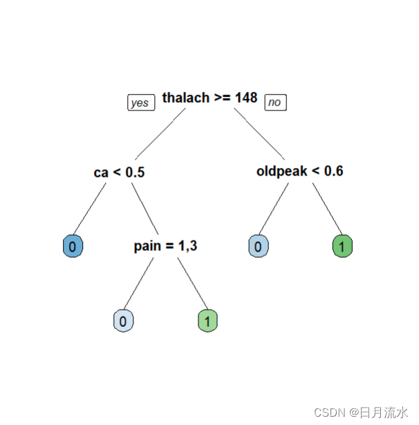
绘制决策树图
fancyRpartPlot(fit.tree,type=5,digits=3,main = '',sub='')

prp(fit.tree,box.palette = 'auto',roundint = FALSE)
3、使用验证数据集分类准确率对决策树进行修剪,选取合适的子树
初始化变量,赋初值
nsubtree<-length(fit.tree$cptable[,1])
results<-data.frame(cp=rep(0,nsubtree),accu=rep(0,nsubtree))
循环的思想是用建立的决策树fit.tree中子树矩阵每个子树对应的复杂度参数CP去修剪决策树,得到每个修剪后的子树,用这些修剪后的子树去验证分层随机抽样后的数据集valid,得到了预测概率和分类结果,与实际真值进行比对,得到了预测准确率,数据框results有两列,一列是每个子树的CP值,一个是验证准确率。
for(j in 1:nsubtree){
results$cp[j]<-fit.tree$cptable[j,'CP']
fit.subtree<-prune(fit.tree,results$cp[j])
prob_valid<-predict(fit.subtree,valid[,-14],
type='prob')[,2]
class_valid<-1*(prob_valid>0.5)
results$accu[j]<-length(which(valid$target2==class_valid))/length(valid$target2)
}
从results数据框中的accu找出最准确的值对于的CP参数值。
bestcp<-results$cp[which.max(results$accu)]
用这个CP参数值进行修剪子树,得到了最佳修剪后子树
fit.valid.subtrees<-prune(fit.tree,bestcp)
4、用修剪后的最佳子树做预测
用这个最佳修改子树去预测测试数据集heart_test,得到了预测概率
prob.tree.valid<-predict(fit.valid.subtrees,heart_test[,-14],type='prob')[,2]
class.tree<-1*(prob.tree>0.5)
得到了分类预测结果
class.tree
得到了预测值和真实值的列联表
table(heart_test$target2,class.tree)
 class.tree
     0  1
  0 34 14
  1 10 33
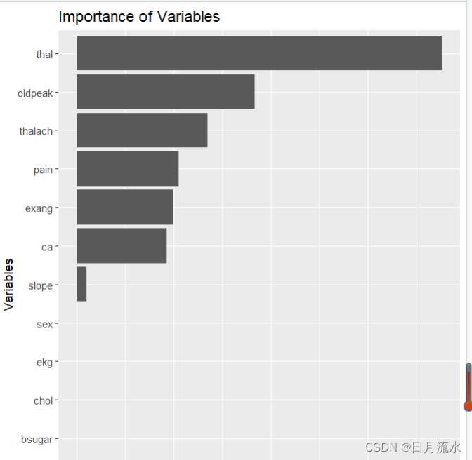
5、每个自变量的影响程度分析
初始化向量importance.tree
importance.tree<-rep(0,13)
names(importance.tree)<-colnames(heart_learning)[1:13]
nvar<-length(fit.valid.subtrees$variable.importance)
通过循环把最佳决策子树中的向量fit.valid.subtrees$variable.importance赋值到向量importance.tree
for(i in 1:nvar)
{ importance.tree[which(names(importance.tree)==names(fit.valid.subtrees$variable.importance)[i])]<-fit.valid.subtrees$variable.importance[i]}
进行标准化
importance.tree<-importance.tree/sum(importance.tree)
imp<-data.frame(name=names(importance.tree),importance=importance.tree)
绘制各变量影响程度的柱形图
ggplot(imp,aes(reorder(name,importance),importance))+geom_col()+xlab('Variables')+
ylab('relative importance')+coord_flip()+ggtitle('Importance of Variables')
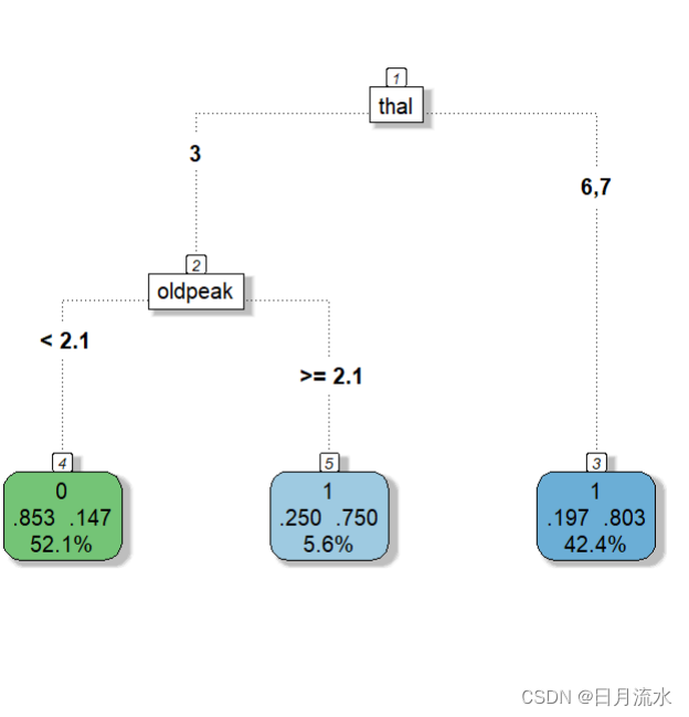
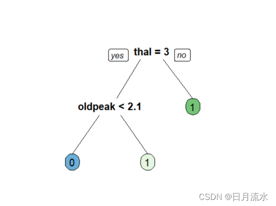
6、查看最佳子树的可视化图形
fancyRpartPlot(fit.valid.subtrees,type=5,digits=3,main = '',sub='')
prp(fit.valid.subtrees,box.palette = 'auto',roundint = FALSE)
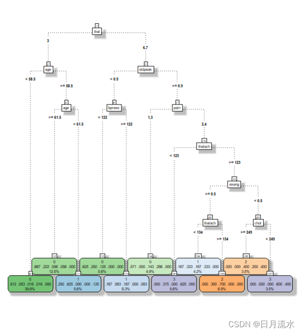
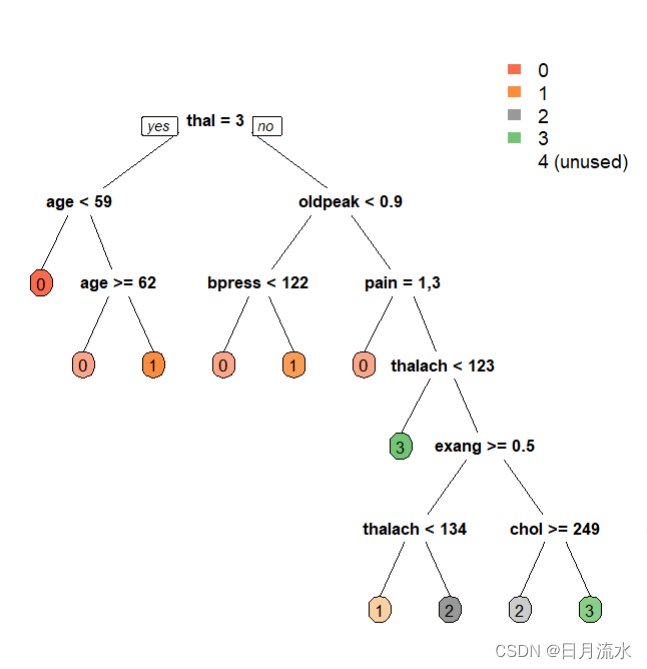
二、对二多值因变量target进行预测
target取值为0,1,2,3,4,程序和target2类似,也需要把分类变量转化为因子变量,需要注意的是预测概率和预测分类类别的取值和定义。
library(rpart)
library(rpart.plot)
library(rattle)
library(dplyr)
library(ggplot2)
library(sampling)
set.seed(12345)
heart_learning<-read.csv('F:/桌面/练习表格/heart_learning.csv',
colClasses=rep('numeric',15)) %>%
mutate(pain=as.factor(pain)) %>% mutate(ekg=as.factor(ekg)) %>%
mutate(slope=as.factor(slope)) %>% mutate(thal=as.factor(thal))
heart_test<-read.csv('F:/桌面/练习表格/heart_test.csv',
colClasses=rep('numeric',15)) %>%
mutate(pain=as.factor(pain)) %>% mutate(ekg=as.factor(ekg)) %>%
mutate(slope=as.factor(slope)) %>% mutate(thal=as.factor(thal))
idtrain<-strata(heart_learning,stratanames = 'target2',
size = round(0.7*table(heart_learning$target)),
method='srswor')$ID_unit
train<-heart_learning[idtrain,]
valid<-heart_learning[-idtrain,]
fit.tree<-rpart(as.factor(target)~.,train[,-15],
parms=list(split='gini'),
control = rpart.control(
minbucket = 5,
minsplit=10,
maxcompete=2,
maxdepth=30,
maxsurrogate=5,
cp=0.0001))
attributes(fit.tree)
print(fit.tree$cptable)
print(fit.tree)
plotcp(fit.tree)
fancyRpartPlot(fit.tree,type=5,digits=3,main = '',sub='')
prp(fit.tree,box.palette = 'auto',roundint = FALSE)
nsubtree<-length(fit.tree$cptable[,1])
results<-data.frame(cp=rep(0,nsubtree),accu=rep(0,nsubtree))
for(j in 1:nsubtree){
results$cp[j]<-fit.tree$cptable[j,'CP']
fit.subtree<-prune(fit.tree,results$cp[j])
prob_valid<-predict(fit.subtree,valid[,-15],
type='prob')
class_valid<-apply(prob_valid,1,which.max)-1
results$accu[j]<-length(which(valid$target==class_valid))/length(valid$target)
}
bestcp<-results$cp[which.max(results$accu)]
fit.valid.subtrees<-prune(fit.tree,bestcp)
importance.tree<-rep(0,13)
names(importance.tree)<-colnames(heart_learning)[1:13]
nvar<-length(fit.valid.subtrees$variable.importance)
for(i in 1:nvar){
importance.tree[which(names(importance.tree)==names(fit.valid.subtrees$variable.importance)[i])]<-fit.valid.subtrees$variable.importance[i]}
importance.tree<-importance.tree/sum(importance.tree)
imp<-data.frame(name=names(importance.tree),importance=importance.tree)
ggplot(imp,aes(reorder(name,importance),importance))+geom_col()+xlab('Variables')+
ylab('relative importance')+coord_flip()+ggtitle('Importance of Variables')
prob.tree<-predict(fit.valid.subtrees,heart_test[,1:13],type = 'prob')
class.tree<-apply(prob.tree,1,which.max)-1
class.tree
table(heart_test$target,class.tree)
运行可以得到
真实值与预测值的列联表
table(heart_test$target,class.tree)
   class.tree
     0  1  2  3
  0 43  4  1  0
  1 10  4  1  2
  2  4  2  3  2
  3  3  4  3  1
  4  1  0  3  0
变量的重要程度柱形图

决策树的可视化图形等