uni-app开发微信小程序获取手机号getPhoneNumber:fail no permission 怎么处理？

一、介绍

        在瞬息万变的金融市场中，准确的预测就像圣杯一样。当我们寻求更复杂的技术来解释市场趋势时，机器学习成为希望的灯塔。在各种机器学习模型中，长短期记忆（LSTM）网络受到了极大的关注。当与注意力机制相结合时，这些模型变得更加强大，尤其是在分析股票价格等时间序列数据时。本文深入探讨了LSTM网络与注意力机制相结合的有趣世界，重点利用雅虎财经（yfinance）的数据预测苹果公司（AAPL）股价接下来的四根蜡烛的模式。所有数据都在这里。

二、第 1 部分：了解 LSTM 和财务建模中的注意

2.1 LSTM 网络的基础知识

        LSTM 网络是一种递归神经网络 （RNN），专门设计用于长时间记忆和处理数据序列。LSTM 与传统 RNN 的区别在于它们能够长时间保存信息，这要归功于其独特的结构，包括三个门：输入门、忘记门和输出门。这些门协同管理信息流，决定保留什么和丢弃什么，从而缓解梯度消失的问题——这是标准 RNN 中的常见问题。

        在金融市场的背景下，这种记住和利用长期依赖关系的能力是无价的。例如，股票价格不仅受到近期趋势的影响，还受到随着时间的推移建立的模式的影响。LSTM 网络能够熟练地捕获这些时间依赖关系，使其成为金融时间序列分析的理想选择。

2.2 注意机制：增强LSTM

        注意力机制最初在自然语言处理领域普及，现已进入包括金融在内的其他各个领域。它基于一个简单而深刻的概念：并非输入序列的所有部分都同样重要。通过允许模型专注于输入序列的特定部分而忽略其他部分，注意力机制增强了模型的上下文理解能力。

        将注意力整合到 LSTM 网络中会产生更集中和上下文感知的模型。在预测股票价格时，某些历史数据点可能比其他数据点更相关。注意力机制使 LSTM 能够更严格地权衡这些点，从而做出更准确和细致的预测。

2.3 金融模式预测的相关性

        LSTM与注意力机制的结合为金融模式预测创造了一个强大的模型。金融市场是一个复杂的适应性系统，受多种因素影响，并表现出非线性特征。传统模型往往无法捕捉到这种复杂性。然而，LSTM网络，特别是当与注意力机制相结合时，善于解开这些模式，提供对未来股票走势的更深入理解和更准确的预测。

        当我们继续构建和实施具有注意力机制的 LSTM 来预测 AAPL 股票接下来的四根蜡烛时，我们深入研究了一个复杂的财务分析领域，该领域有望彻底改变我们如何解释和应对不断变化的股票市场动态。

三、第 2 部分：设置环境

        要开始构建我们的 LSTM 模型并注意预测 AAPL 股票模式，第一步是在 Google Colab 中设置我们的编码环境。Google Colab 提供基于云的服务，提供免费的 Jupyter 笔记本环境，支持 GPU，非常适合运行深度学习模型。

！pip install tensorflow -qqq
！pip install keras -qqq
！pip install yfinance -qqq

3.1 设置环境

        安装后，我们可以将这些库导入到我们的 Python 环境中。运行以下代码：

import tensorflow as tf
import keras
import yfinance as yf
import numpy as np
import pandas as pd
import matplotlib.pyplot as plt

# Check TensorFlow version
print("TensorFlow Version: ", tf.__version__)

        此代码不仅导入库，还检查 TensorFlow 版本以确保所有内容都是最新的。

3.2 yfinance的数据采集

2.2.1 获取历史数据

        要分析 AAPL 股票模式，我们需要历史股价数据。这就是 yfinance 发挥作用的地方。该库旨在从雅虎财经获取历史市场数据。

3.2.2. 数据下载代码

在 Colab 笔记本中运行以下代码以下载 AAPL 的历史数据：

# Fetch AAPL data
aapl_data = yf.download('AAPL', start='2020-01-01', end='2024-01-01')

# Display the first few rows of the dataframe
aapl_data.head()

        此脚本获取 Apple Inc. 从 2020 年 1 月 1 日到 2024 年 1 月 1 日的每日股价。您可以根据自己的喜好调整开始日期和结束日期。

3.3 数据预处理和特征选择的重要性

        获取数据后，预处理和特征选择变得至关重要。预处理涉及清理数据并使其适合模型。这包括处理缺失值、规范化或缩放数据，以及可能创建其他特征，如移动平均值或百分比变化，以帮助模型更有效地学习。

        特征选择是关于选择对预测变量贡献最大的正确特征集。对于股票价格预测，通常使用开盘价、收盘价、最高价、最低价和成交量等特征。选择提供相关信息的特征以防止模型从噪声中学习非常重要。

在接下来的章节中，我们将对这些数据进行预处理，并使用注意力层构建 LSTM 模型以开始进行预测。

四、第 3 部分：数据预处理和准备

        在构建 LSTM 模型之前，第一个关键步骤是准备我们的数据集。本节介绍了数据预处理的基本阶段，以使 yfinance 的 AAPL 股票数据为我们的 LSTM 模型做好准备。

4.1 数据清理

        股票市场数据集通常包含异常或缺失值。处理这些问题以防止预测不准确至关重要。

• 识别缺失值：检查数据集中是否有任何缺失数据。如果有，您可以选择使用正向填充或向后填充等方法填充它们，或者完全删除这些行。

# Checking for missing values
aapl_data.isnull().sum()

# Filling missing values, if any
aapl_data.fillna(method='ffill', inplace=True)

• 处理异常：有时，由于数据收集中的故障，数据集包含错误的值。如果您发现任何异常情况（例如不切实际的股价极端飙升），则应纠正或删除它们。

4.2 功能选择

        在股票市场数据中，各种特征都可能具有影响力。通常使用“开盘价”、“最高价”、“最低价”、“收盘价”和“成交量”。

• 决定功能：对于我们的模型，我们将使用“收盘价”，但您可以尝试使用其他功能，例如“开盘价”、“最高价”、“最低价”和“成交量”。

4.3 正常化

        归一化是一种用于将数据集中数值列的值更改为通用比例的技术，而不会扭曲值范围的差异。

• 应用最小-最大缩放：这将缩放数据集，使所有输入要素都位于 0 和 1 之间。

from sklearn.preprocessing import MinMaxScaler

scaler = MinMaxScaler(feature_range=(0,1))
aapl_data_scaled = scaler.fit_transform(aapl_data['Close'].values.reshape(-1,1))

4.4 创建序列

LSTM 模型要求输入采用序列格式。我们将数据转换为序列，供模型学习。

• 定义序列长度：选择序列长度（如 60 天）。这意味着，对于每个样本，模型将查看过去 60 天的数据以做出预测。

X = []
y = []

for i in range(60, len(aapl_data_scaled)):
    X.append(aapl_data_scaled[i-60:i, 0])
    y.append(aapl_data_scaled[i, 0])

4.5 训练-测试拆分

将数据拆分为训练集和测试集，以正确评估模型的性能。

• 定义拆分率：通常，80% 的数据用于训练，20% 用于测试。

train_size = int(len(X) * 0.8)
test_size = len(X) - train_size

X_train, X_test = X[:train_size], X[train_size:]
y_train, y_test = y[:train_size], y[train_size:]

4.6 重塑 LSTM 的数据

        最后，我们需要将数据重塑为 LSTM 图层所需的 3D 格式。[samples, time steps, features]

• 重塑数据：

X_train, y_train = np.array(X_train), np.array(y_train)
X_train = np.reshape(X_train, (X_train.shape[0], X_train.shape[1], 1))

在下一节中，我们将利用这些预处理的数据来构建和训练具有注意力机制的 LSTM 模型。

五、第 4 部分：使用注意力模型构建 LSTM

在本节中，我们将深入探讨 LSTM 模型的构建，该模型具有额外的注意力机制，专为预测 AAPL 股票模式而量身定制。这需要 TensorFlow 和 Keras，它们应该已经在 Colab 环境中设置好了。

5.1 创建 LSTM 图层

        我们的 LSTM 模型将由多个层组成，包括用于处理时间序列数据的 LSTM 层。基本结构如下：

from keras.models import Sequential
from keras.layers import LSTM, Dense, Dropout, AdditiveAttention, Permute, Reshape, Multiply

model = Sequential()

# Adding LSTM layers with return_sequences=True
model.add(LSTM(units=50, return_sequences=True, input_shape=(X_train.shape[1], 1)))
model.add(LSTM(units=50, return_sequences=True))

在此模型中，表示每个 LSTM 层中的神经元数。 unitsreturn_sequences=True在第一层中至关重要，以确保输出包含序列，这对于堆叠 LSTM 层至关重要。当我们为注意力层准备数据时，最终的 LSTM 层不会返回序列。

5.2 整合注意力机制

        可以添加注意力机制来增强模型关注相关时间步长的能力：

# Adding self-attention mechanism
# The attention mechanism
attention = AdditiveAttention(name='attention_weight')
# Permute and reshape for compatibility
model.add(Permute((2, 1))) 
model.add(Reshape((-1, X_train.shape[1])))
attention_result = attention([model.output, model.output])
multiply_layer = Multiply()([model.output, attention_result])
# Return to original shape
model.add(Permute((2, 1))) 
model.add(Reshape((-1, 50)))

# Adding a Flatten layer before the final Dense layer
model.add(tf.keras.layers.Flatten())

# Final Dense layer
model.add(Dense(1))

# Compile the model
# model.compile(optimizer='adam', loss='mean_squared_error')

# Train the model
# history = model.fit(X_train, y_train, epochs=100, batch_size=25, validation_split=0.2)

        此自定义层计算输入序列的加权总和，使模型能够更加关注某些时间步长。

5.3 优化模型

        为了提高模型的性能并降低过拟合的风险，我们包括了 Dropout 和 Batch Normalization。

from keras.layers import BatchNormalization

# Adding Dropout and Batch Normalization
model.add(Dropout(0.2))
model.add(BatchNormalization())

        在训练期间，每次更新时，Dropout 都会将一部分输入单位随机设置为 0，从而有助于防止过拟合，而批量归一化则稳定了学习过程。

5.4 模型编译

        最后，我们使用适合回归任务的优化器和损失函数编译模型。

model.compile(optimizer='adam', loss='mean_squared_error')

  adam优化器通常是递归神经网络的不错选择，而均方误差可以很好地用作像我们这样的回归任务的损失函数。

5.5 模型摘要

查看模型的摘要以了解其结构和参数数是有益的。

model.summary()

六、第 5 部分：训练模型

        现在，我们的 LSTM 模型已经构建好了，是时候使用我们准备好的训练集来训练它了。此过程涉及将训练数据提供给模型并让它学习进行预测。

6.1 培训代码

        使用以下代码使用 X_train和 y_train训练模型：

# Assuming X_train and y_train are already defined and preprocessed
history = model.fit(X_train, y_train, epochs=100, batch_size=25, validation_split=0.2)

        在这里，我们训练 100 个 epoch 的模型，批处理大小为 25。该参数保留了一部分训练数据进行验证，validation_split使我们能够在训练期间监控模型在看不见的数据上的性能。

6.2 过拟合以及如何避免过拟合

        当模型学习特定于训练数据的模式时，就会发生过拟合，这些模式不会泛化到新数据。以下是避免过度拟合的方法：

1. 验证集：使用验证集（正如我们在训练代码中所做的那样）有助于监控模型在看不见的数据上的性能。
2. 提前停止：当模型在验证集上的性能开始下降时，此技术将停止训练。在 Keras 中实现提前停止很简单：

from keras.callbacks import EarlyStopping

early_stopping = EarlyStopping(monitor='val_loss', patience=10)
history = model.fit(X_train, y_train, epochs=100, batch_size=25, validation_split=0.2, callbacks=[early_stopping])

1. 在这里，如果验证损失连续 10 个周期没有改善，则表示训练将停止。patience=10
2. 正则化技术：像 Dropout 和 Batch Normalization 这样的技术已经包含在我们的模型中，也有助于减少过拟合。

可选：这些是更多回调

from keras.callbacks import ModelCheckpoint, ReduceLROnPlateau, TensorBoard, CSVLogger

# Callback to save the model periodically
model_checkpoint = ModelCheckpoint('best_model.h5', save_best_only=True, monitor='val_loss')

# Callback to reduce learning rate when a metric has stopped improving
reduce_lr = ReduceLROnPlateau(monitor='val_loss', factor=0.1, patience=5)

# Callback for TensorBoard
tensorboard = TensorBoard(log_dir='./logs')

# Callback to log details to a CSV file
csv_logger = CSVLogger('training_log.csv')

# Combining all callbacks
callbacks_list = [early_stopping, model_checkpoint, reduce_lr, tensorboard, csv_logger]

# Fit the model with the callbacks
history = model.fit(X_train, y_train, epochs=100, batch_size=25, validation_split=0.2, callbacks=callbacks_list)

七、第 6 部分：评估模型性能

        训练模型后，下一步是使用测试集评估其性能。这将使我们了解我们的模型可以很好地推广到新的、看不见的数据。

7.1 使用测试集进行评估

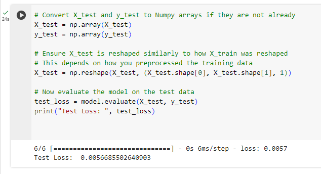
        为了评估模型，我们首先需要准备测试数据X_test（），就像我们对训练数据所做的那样。然后，我们可以使用模型的函数：​​​​​​​evaluate

# Convert X_test and y_test to Numpy arrays if they are not already
X_test = np.array(X_test)
y_test = np.array(y_test)

# Ensure X_test is reshaped similarly to how X_train was reshaped
# This depends on how you preprocessed the training data
X_test = np.reshape(X_test, (X_test.shape[0], X_test.shape[1], 1))

# Now evaluate the model on the test data
test_loss = model.evaluate(X_test, y_test)
print("Test Loss: ", test_loss)

7.2 性能指标

        除了损失之外，其他指标还可以提供对模型性能的更多见解。对于像我们这样的回归任务，常见指标包括：

1. 平均绝对误差 （MAE）：它测量一组预测中误差的平均幅度，而不考虑其方向。
2. 均方根误差 （RMSE）：这是预测和实际观测值之间平方差平均值的平方根。

为了计算这些指标，我们可以使用我们的模型进行预测，并将它们与实际值进行比较：

from sklearn.metrics import mean_absolute_error, mean_squared_error

# Making predictions
y_pred = model.predict(X_test)

# Calculating MAE and RMSE
mae = mean_absolute_error(y_test, y_pred)
rmse = mean_squared_error(y_test, y_pred, squared=False)

print("Mean Absolute Error: ", mae)
print("Root Mean Square Error: ", rmse)

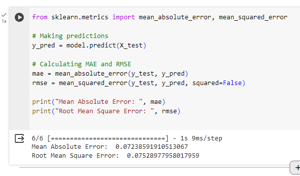
型：

• 平均绝对误差 （MAE）：0.0724（大约）
• 均方根误差 （RMSE）：0.0753（近似值）

        MAE 和 RMSE 都是回归模型预测准确性的度量。以下是他们所指出的：

        MAE 测量一组预测中误差的平均幅度，而不考虑其方向。它是预测和实际观察之间绝对差异的检验样本的平均值，其中所有个体差异的权重相等。MAE 为 0.0724 意味着平均而言，模型的预测值与实际值相差约 0.0724 个单位。

        RMSE 是一种二次评分规则，也测量误差的平均幅度。它是预测值和实际观测值之间差值平方值的平方根。RMSE对大误差的权重相对较高。这意味着当大错误特别不受欢迎时，RMSE 应该更有用。RMSE 为 0.0753 意味着当误差越大受到惩罚时，模型的预测平均与实际值相差 0.0753 个单位。

        这些指标将帮助您了解模型的准确性以及需要改进的地方。通过分析这些指标，您可以就进一步调整模型或更改方法做出明智的决策。

        在下一节中，我们将讨论如何使用该模型进行实际的库存模式预测，以及将此模型部署到实际应用中的实际注意事项。

八、第 7 部分：预测接下来的 4 根蜡烛

        在用注意力机制训练和评估了我们的 LSTM 模型后，最后一步是利用它来预测 AAPL 股价接下来的 4 根蜡烛（天）。

8.1 做出预测

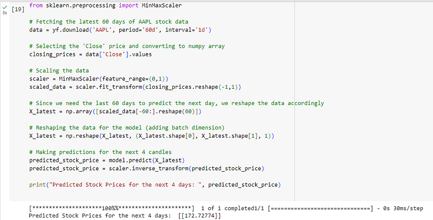
        为了预测未来的股票价格，我们需要为模型提供最新的数据点。假设我们准备了最近 60 天的数据，格式与 ： 相同，并且我们想要预测第二天的价格：X_train

import yfinance as yf
import numpy as np
from sklearn.preprocessing import MinMaxScaler

# Fetching the latest 60 days of AAPL stock data
data = yf.download('AAPL', period='60d', interval='1d')

# Selecting the 'Close' price and converting to numpy array
closing_prices = data['Close'].values

# Scaling the data
scaler = MinMaxScaler(feature_range=(0,1))
scaled_data = scaler.fit_transform(closing_prices.reshape(-1,1))

# Since we need the last 60 days to predict the next day, we reshape the data accordingly
X_latest = np.array([scaled_data[-60:].reshape(60)])

# Reshaping the data for the model (adding batch dimension)
X_latest = np.reshape(X_latest, (X_latest.shape[0], X_latest.shape[1], 1))

# Making predictions for the next 4 candles
predicted_stock_price = model.predict(X_latest)
predicted_stock_price = scaler.inverse_transform(predicted_stock_price)

print("Predicted Stock Prices for the next 4 days: ", predicted_stock_price)

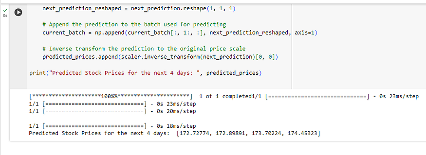
        让我们预测未来 4 天的价格：

import yfinance as yf
import numpy as np
from sklearn.preprocessing import MinMaxScaler

# Fetch the latest 60 days of AAPL stock data
data = yf.download('AAPL', period='60d', interval='1d')

# Select 'Close' price and scale it
closing_prices = data['Close'].values.reshape(-1, 1)
scaler = MinMaxScaler(feature_range=(0, 1))
scaled_data = scaler.fit_transform(closing_prices)

# Predict the next 4 days iteratively
predicted_prices = []
current_batch = scaled_data[-60:].reshape(1, 60, 1)  # Most recent 60 days

for i in range(4):  # Predicting 4 days
    # Get the prediction (next day)
    next_prediction = model.predict(current_batch)
    
    # Reshape the prediction to fit the batch dimension
    next_prediction_reshaped = next_prediction.reshape(1, 1, 1)
    
    # Append the prediction to the batch used for predicting
    current_batch = np.append(current_batch[:, 1:, :], next_prediction_reshaped, axis=1)
    
    # Inverse transform the prediction to the original price scale
    predicted_prices.append(scaler.inverse_transform(next_prediction)[0, 0])

print("Predicted Stock Prices for the next 4 days: ", predicted_prices)

8.2 预测的可视化

        直观地将预测值与实际股票价格进行比较可能会非常有见地。以下是将预测股价与实际数据进行对比的代码：

!pip install mplfinance -qqq
import pandas as pd
import mplfinance as mpf
import matplotlib.dates as mpl_dates
import matplotlib.pyplot as plt

# Assuming 'data' is your DataFrame with the fetched AAPL stock data
# Make sure it contains Open, High, Low, Close, and Volume columns

# Creating a list of dates for the predictions
last_date = data.index[-1]
next_day = last_date + pd.Timedelta(days=1)
prediction_dates = pd.date_range(start=next_day, periods=4)

# Assuming 'predicted_prices' is your list of predicted prices for the next 4 days
predictions_df = pd.DataFrame(index=prediction_dates, data=predicted_prices, columns=['Close'])

# Plotting the actual data with mplfinance
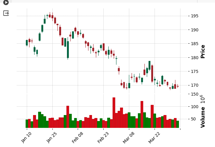
mpf.plot(data, type='candle', style='charles', volume=True)

# Overlaying the predicted data
plt.figure(figsize=(10,6))
plt.plot(predictions_df.index, predictions_df['Close'], linestyle='dashed', marker='o', color='red')

plt.title("AAPL Stock Price with Predicted Next 4 Days")
plt.show()

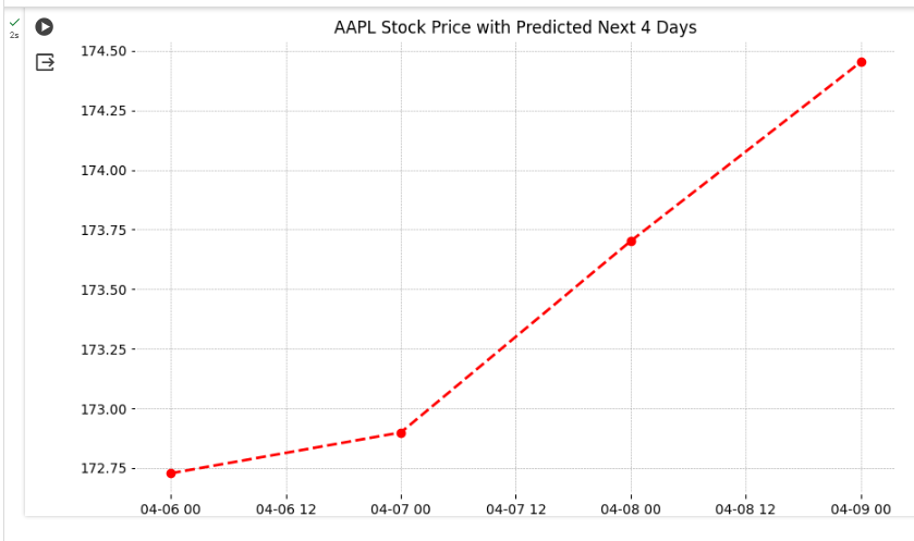
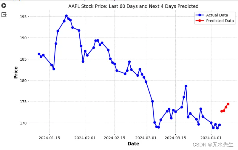
8.3 预测的最终视觉对象：

import pandas as pd
import mplfinance as mpf
import matplotlib.dates as mpl_dates
import matplotlib.pyplot as plt

# Fetch the latest 60 days of AAPL stock data
data = yf.download('AAPL', period='64d', interval='1d') # Fetch 64 days to display last 60 days in the chart

# Select 'Close' price and scale it
closing_prices = data['Close'].values.reshape(-1, 1)
scaler = MinMaxScaler(feature_range=(0, 1))
scaled_data = scaler.fit_transform(closing_prices)

# Predict the next 4 days iteratively
predicted_prices = []
current_batch = scaled_data[-60:].reshape(1, 60, 1)  # Most recent 60 days

for i in range(4):  # Predicting 4 days
    next_prediction = model.predict(current_batch)
    next_prediction_reshaped = next_prediction.reshape(1, 1, 1)
    current_batch = np.append(current_batch[:, 1:, :], next_prediction_reshaped, axis=1)
    predicted_prices.append(scaler.inverse_transform(next_prediction)[0, 0])

# Creating a list of dates for the predictions
last_date = data.index[-1]
next_day = last_date + pd.Timedelta(days=1)
prediction_dates = pd.date_range(start=next_day, periods=4)

# Adding predictions to the DataFrame
predicted_data = pd.DataFrame(index=prediction_dates, data=predicted_prices, columns=['Close'])

# Combining both actual and predicted data
combined_data = pd.concat([data['Close'], predicted_data['Close']])
combined_data = combined_data[-64:] # Last 60 days of actual data + 4 days of predictions

# Plotting the actual data
plt.figure(figsize=(10,6))
plt.plot(data.index[-60:], data['Close'][-60:], linestyle='-', marker='o', color='blue', label='Actual Data')

# Plotting the predicted data
plt.plot(prediction_dates, predicted_prices, linestyle='-', marker='o', color='red', label='Predicted Data')

plt.title("AAPL Stock Price: Last 60 Days and Next 4 Days Predicted")
plt.xlabel('Date')
plt.ylabel('Price')
plt.legend()
plt.show()

九、结论

        在本指南中，我们探讨了将 LSTM 网络与注意力机制用于股价预测的复杂而迷人的任务，特别是针对 Apple Inc. （AAPL）。关键点包括：

• LSTM 捕获时间序列数据中长期依赖关系的能力。
• 注意力机制在关注相关数据点方面的额外优势。
• 构建、训练和评估 LSTM 模型的详细过程。

        虽然具有注意力的 LSTM 模型功能强大，但它们也有局限性：

• 假设历史模式将以类似的方式重演可能会有问题，尤其是在动荡的市场中。
• 历史价格数据中没有捕捉到的外部因素，如市场新闻和全球事件，可以显着影响股价。