github生成新的SSH密钥

一、环境搭建

Links for tensorflow-gpu (tsinghua.edu.cn)

验证环境是否成功的测试代码：

from keras.datasets import mnist  ##从keras中导入mnist数据集,图片像素是28*28
from keras import models
from keras import layers
from keras.utils import to_categorical ##用于标签

#导入数据集
(train_images,train_labels),(test_images,test_labels)=mnist.load_data()##得到的是numpy数组
print(train_images.shape)##60000张图片，28*28像素大小

#定义网络
network=models.Sequential()
network.add(layers.Dense(512,activation='relu',input_shape=(28*28,)))##Dense为全连接层
network.add(layers.Dense(10,activation='softmax'))
network.compile(optimizer='rmsprop',loss='categorical_crossentropy',metrics=['accuracy'])
##改变训练数据集形状
train_images=train_images.reshape((60000,28*28))
train_images=train_images.astype('float32')/255
#改变测试集形状
test_images=test_images.reshape((10000,28*28))
test_images=test_images.astype('float32')/255
#设置标签
train_labels=to_categorical(train_labels)
test_labels=to_categorical(test_labels)
##训练网络，使用fit函数
network.fit(train_images,train_labels,epochs=5,batch_size=128)

##查看在测试集上的效果
test_loss,test_acc=network.evaluate(test_images,test_labels)
print('test_acc',test_acc)##输出在测试集上的精度

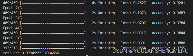
 运行陈工的结果如下图所示：

二、手写体数据下载

下载代码

"""
下载MNIST数据集脚本
"""

import os
from pathlib import Path
import logging

import wget

logging.basicConfig(level=logging.INFO, format="%(message)s")


def download_minst(save_dir: str = None) -> bool:
    """下载MNIST数据集
    输入参数:
        save_dir: MNIST数据集的保存地址. 类型: 字符串.

    返回值:
        全部下载成功返回True, 否则返回False
    """
    
    save_dir = Path(save_dir)
    train_set_imgs_addr = save_dir / "train-images-idx3-ubyte.gz"
    train_set_labels_addr = save_dir / "train-labels-idx1-ubyte.gz"
    test_set_imgs_addr = save_dir / "t10k-images-idx3-ubyte.gz"
    test_set_labels_addr = save_dir / "t10k-labels-idx1-ubyte.gz"

    try:
        if not os.path.exists(train_set_imgs_addr):
            logging.info("下载train-images-idx3-ubyte.gz")
            filename = wget.download(url="http://yann.lecun.com/exdb/mnist/train-images-idx3-ubyte.gz", out=str(train_set_imgs_addr))
            logging.info("\tdone.")
        else:
            logging.info("train-images-idx3-ubyte.gz已经存在.")

        if not os.path.exists(train_set_labels_addr):
            logging.info("下载train-labels-idx1-ubyte.gz.")
            filename = wget.download(url="http://yann.lecun.com/exdb/mnist/train-labels-idx1-ubyte.gz", out=str(train_set_labels_addr))
            logging.info("\tdone.")
        else:
            logging.info("train-labels-idx1-ubyte.gz已经存在.")

        if not os.path.exists(test_set_imgs_addr):
            logging.info("下载t10k-images-idx3-ubyte.gz.")
            filename = wget.download(url="http://yann.lecun.com/exdb/mnist/t10k-images-idx3-ubyte.gz", out=str(test_set_imgs_addr))
            logging.info("\tdone.")
        else:
            logging.info("t10k-images-idx3-ubyte.gz已经存在.")

        if not os.path.exists(test_set_labels_addr):
            logging.info("下载t10k-labels-idx1-ubyte.gz.")
            filename = wget.download(url="http://yann.lecun.com/exdb/mnist/t10k-labels-idx1-ubyte.gz", out=str(test_set_labels_addr))
            logging.info("\tdone.")
        else:
            logging.info("t10k-labels-idx1-ubyte.gz已经存在.")
        
    except:
        return False
    
    return True


if __name__ == "__main__":
	download_minst(save_dir="/home/kongxianglan/sim_code/")

直接下载数据包的方法：点击下面的链接能够直接下载

https://s3.amazonaws.com/img-datasets/mnist.npz

三、手写体图像相似性对比方法一

参考代码的链接：孪生网络keras实现minist_keras minist-CSDN博客

 该代码是基于手写体压缩包的，如果要更换为自己的图像或者单张图像测试，修改起来比较麻烦。整个代码如下：

注意这里的数据集加载的直接是一个压缩包，数据的下载地址为：

https://s3.amazonaws.com/img-datasets/mnist.npz

1）训练及模型保存

import numpy as np
import keras
from keras.layers import *

path = 'siameseData.npz'
f = np.load(path)

x1, x2, Y = f["x1"], f['x2'], f['Y']
x1 = x1.astype('float32')/255.
x2 = x2.astype('float32')/255.
x1 = x1.reshape(60000,28,28,1)
print(x2.shape)
x2 = x2.reshape(60000,28,28,1)
print(Y.shape)



# ---------------------查看相同数字（不同数字）个数----------------------
def sum():
    oneSum = 0
    zerosSum = 0
    for i in range(60000):
        if Y[i] == 1:
            oneSum = oneSum + 1
        else:
            zerosSum = zerosSum + 1
    print("相同的个数{}".format(oneSum))
    print("不同的个数{}".format(zerosSum))


sum()  # 相同的个数30000，不同的个数30000


# ---------------------查看相同数字（不同数字）个数----------------------


# -----------------------开始孪生网络构建--------------------------------------

# 特征提取，对两张图片进行特征提取
def FeatureNetwork():
    F_input = Input(shape=(28, 28, 1), name='FeatureNet_ImageInput')

    # ----------------------------------网络第一层----------------------
    # 28,28,1-->28,28,24
    models = Conv2D(filters=24, kernel_size=(3, 3), strides=1, padding='same')(F_input)
    models = Activation('relu')(models)
    # 28,28,24-->9,9,24
    models = MaxPooling2D(pool_size=(3, 3))(models)
    # ----------------------------------网络第一层----------------------

    # ----------------------------------网络第二层----------------------
    # 9,9,24-->9,9,64
    models = Conv2D(filters=64, kernel_size=(3, 3), strides=1, padding='same')(models)
    models = Activation('relu')(models)
    # ----------------------------------网络第二层----------------------

    # ----------------------------------网络第三层----------------------
    # 9,9,64-->7,7,96
    models = Conv2D(filters=96, kernel_size=(3, 3), strides=1, padding='valid')(models)
    models = Activation('relu')(models)
    # ----------------------------------网络第三层----------------------

    # ----------------------------------网络第四层----------------------
    # 7,7,96-->5,5,96
    models = Conv2D(filters=96, kernel_size=(3, 3), strides=1, padding='valid')(models)
    # ----------------------------------网络第四层----------------------

    # ----------------------------------网络第五层----------------------
    # 5,5,96-->2400
    models = Flatten()(models)
    # 2400-->512
    models = Dense(512)(models)
    models = Activation('relu')(models)
    # ----------------------------------网络第五层----------------------

    return keras.Model(F_input, models)


# 共享参数
def ClassifilerNet():
    model = FeatureNetwork()
    inp1 = Input(shape=(28, 28, 1))  # 创建输入
    inp2 = Input(shape=(28, 28, 1))  # 创建输入2
    model_1 = model(inp1)  # 孪生网络中的一个特征提取分支
    model_2 = model(inp2)  # 孪生网络中的另一个特征提取分支
    merge_layers = concatenate([model_1, model_2])  # 进行融合，使用的是默认的sum，即简单的相加
    # ----------全连接---------
    fc1 = Dense(1024, activation='relu')(merge_layers)
    fc2 = Dense(256, activation='relu')(fc1)
    fc3 = Dense(1, activation='sigmoid')(fc2)

    # ----------构建最终网络
    class_models = keras.Model([inp1, inp2], fc3)  # 最终网络架构，特征层+全连接层
    return class_models


#-----------------------孪生网络实例化以及编译训练-----------------------
siamese_model = ClassifilerNet()
siamese_model.summary()


siamese_model.compile(loss='mse', # 损失函数采用mse
                      optimizer='rmsprop',
                      metrics=['accuracy']
                      )



history = siamese_model.fit([x1,x2],Y,
                            batch_size=256,
                            epochs=100,
                            validation_split=0.2)


#-----------------------孪生网络实例化以及编译训练end-----------------------
siamese_model.save('siamese_model2.h5')
print(history.history.keys())

# ----------------------查看效果-------------------------------
import matplotlib.pyplot as plt
# 准确
plt.plot(history.history['accuracy']) # 训练集准确率
plt.plot(history.history['val_accuracy']) # 验证集准确率
plt.legend()
plt.show()
# 画损失
plt.plot(history.history['loss'])
plt.plot(history.history['val_loss'])
plt.legend()
plt.show()

 2）使用训练的模型进行推理

import keras
import numpy as np
import matplotlib.pyplot as plt

'''
frist（）中的数据集是siameseData.npz中的，即没有验证集，
second（）中有创建了一个数据集，当做验证集（siameseData2.npz），也就是在运行一遍3数据集制作
的代码，把里面的siameseData.npz改为siameseData2.npz便可
'''
def first():
    path = 'siameseData.npz'
    f = np.load(path)

    x1, x2, Y = f["x1"], f['x2'], f['Y']
    x = []
    y = []
    id = 0
    # 找10个数字相同的组成数据集，然后测试，理论输出全是1，（如有意外，纯属理论不够）
    for i in range(len(Y)):
        if id<10:
            if Y[i] == 1:
                x.append(x1[i])
                y.append(x2[i])
                id = id+1

    x = np.asarray(x)
    y = np.asarray(y)
    x = x.reshape(10,28,28,1)
    y = y.reshape(10,28,28,1)


    model = keras.models.load_model('siamese_model2.h5')
    print(model.predict([x,y]))


# 可以在制作一个测试集
def second():
    path = 'siameseData.npz'
    f = np.load(path)

    x1, x2, Y = f["x1"], f['x2'], f['Y']
    # 数据处理
    x1 = x1.reshape(60000,28,28,1)
    x2 = x2.reshape(60000,28,28,1)
    # 查看准确率
    model = keras.models.load_model('siamese_model2.h5')
    print(model.evaluate([x1,x2],Y))

    # second() # 准确率大概97.49%


if __name__ == "__main__":
    # first()
    second()

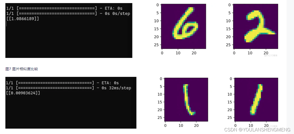
运行结果如图所示：

四、手写体相似性比对方法二 

      孪生神经网络（Siamese neural network），又名双生神经网络，是基于两个人工神经网络建立的耦合构架。孪生神经网络以两个样本为输入，输出其嵌入高维度空间的表征，以比较两个样本的相似程度。狭义的孪生神经网络由两个结构相同，且权重共享的神经网络拼接而成。广义的孪生神经网络，或“伪孪生神经网络（pseudo-siamese network）”，可由任意两个神经网拼接而成。孪生神经网络通常具有深度结构，可由卷积神经网络、循环神经网络等组成。

      所谓权值共享就是当神经网络有两个输入的时候，这两个输入使用的神经网络的权值是共享的（可以理解为使用了同一个神经网络）。很多时候，我们需要去评判两张图片的相似性，比如比较两张人脸的相似性，我们可以很自然的想到去提取这个图片的特征再进行比较，自然而然的，我们又可以想到利用神经网络进行特征提取。如果使用两个神经网络分别对图片进行特征提取，提取到的特征很有可能不在一个域中，此时我们可以考虑使用一个神经网络进行特征提取再进行比较。这个时候我们就可以理解孪生神经网络为什么要进行权值共享了。
      孪生神经网络有两个输入（Input1 and Input2），利用神经网络将输入映射到新的空间，形成输入在新的空间中的表示。通过Loss的计算，评价两个输入的相似度。

参考博文：孪生神经网络 检测 孪生神经网络人脸识别_kekenai的技术博客_51CTO博客

1）MINIST数据集转换为图像

将第二章中，使用代码下载的数据集解压，然后将解压后的minist数据，转换成jpg图像，代码如下：

import os
import idx2numpy
from PIL import Image
from tqdm import tqdm
 
def save_images(images, labels, target_dir):
    for label in range(10):
        label_dir = os.path.join(target_dir, str(label))
        os.makedirs(label_dir, exist_ok=True)
 
        # 获取当前标签的所有图像
        label_images = images[labels == label]
 
        # 为当前标签的每张图像显示进度条
        for i, img in enumerate(tqdm(label_images, desc=f"Processing {target_dir}/{label}", ascii=True)):
            img_path = os.path.join(label_dir, f"{i}.jpg")
            img = Image.fromarray(img)
            img.save(img_path)
 
#! MNIST数据集文件路径
train_img_path="../train-images.idx3-ubyte"
train_lbl_path="../train-labels.idx1-ubyte"
test_img_path="../t10k-images.idx3-ubyte"
test_lbl_path="../t10k-labels.idx1-ubyte"


 
# 读取数据集
train_images = idx2numpy.convert_from_file(train_img_path)
train_labels = idx2numpy.convert_from_file(train_lbl_path)
test_images = idx2numpy.convert_from_file(test_img_path)
test_labels = idx2numpy.convert_from_file(test_lbl_path)
 
# 保存图像
save_images(train_images, train_labels, 'train')
save_images(test_images, test_labels, 'test')

2)重命名以及将重命名的图像放在同一个文件夹中

由于作者要求的数据集的长相如下图所示：

所以我们需要经过以下两个操作将数据集和上图对应在一起

1)重命名

import os
import shutil

import os
import re
import shutil


def get_files(path):
    """ 获取指定路径下所有文件名称 """
    files = []
    for filename in os.listdir(path):
        if os.path.isfile(os.path.join(path, filename)):
            files.append(filename)
    return files


if __name__ == '__main__':
   
 
    number=[0,1,2,3,4,5,6,7,8]

    for index in range (len(number)):
    
        # 指定文件夹路径

        str_number=str(number[index])
    
        folder_path_image = "../test/"+str_number+"/"

        # save_folder_path_image = "../train_new/"
        

        file_list_iamge = os.listdir(folder_path_image)

        
        # 循环遍历每一个文件名并对其进行重命名
        for i, name in enumerate(file_list_iamge):
        
            if not name.endswith('.png') and not name.endswith('.bmp') and not name.endswith('.jpg'):
                continue
                    # 设置新文件名
            new_name = "test_" + str(i).zfill(2) +'_'+ str_number+'.jpg'
            print(new_name)

            os.rename(os.path.join(folder_path_image, name), os.path.join(folder_path_image, new_name))

 2）将文件移动到一个文件夹中

import glob
import cv2
import numpy as np
import os

combine_path = [ '../test/0/',
                			'../test/1/',
                			'../test/2/',
                			'../test/3/',
                			'../test/4/',
                            '../test/5/',
                            '../test/6/',
                            '../test/7/',
                            '../test/8/',
                            '../test/9/',
                            ]


def open_image(path1):
    img_path = glob.glob(path1)
    return np.array([cv2.imread(true_path) for true_path in img_path])

if __name__ == '__main__':
    sum=len(combine_path)
    for index in range(sum):
        file_list_iamge = os.listdir(combine_path[index])
        for i, name in enumerate(file_list_iamge):
            true_path=combine_path[index]+name
            image=cv2.imread(true_path)
            save_path="../test_new/"+name
            cv2.imwrite(save_path,image)
        
          

以上是对测试集的操作，训练集的操作一样的，将test文件夹更换为train即可

3）训练

from keras.layers import Input,Dense  

from keras.layers import Flatten,Lambda,Dropout  

from keras.models import Model  

import keras.backend as K  

from keras.models import load_model  

import numpy as np  

from PIL import Image  

import glob  

import matplotlib.pyplot as plt  

from PIL import Image  

import random  

from keras.optimizers import Adam,RMSprop  

import tensorflow as tf  

#参考网址：https://blog.51cto.com/u_13259/8067915

def create_base_network(input_shape):  

    image_input = Input(shape=input_shape)  

    x = Flatten()(image_input)  

    x = Dense(128, activation='relu')(x)  

    x = Dropout(0.1)(x)  

    x = Dense(128, activation='relu')(x)  

    x = Dropout(0.1)(x)  

    x = Dense(128, activation='relu')(x)  

    model = Model(image_input,x,name = 'base_network')  

    return model  


def contrastive_loss(y_true, y_pred):  

     margin = 1  

     sqaure_pred = K.square(y_pred)  

     margin_square = K.square(K.maximum(margin - y_pred, 0))  

     return K.mean(y_true * sqaure_pred + (1 - y_true) * margin_square)  


def accuracy(y_true, y_pred): # Tensor上的操作  

    return K.mean(K.equal(y_true, K.cast(y_pred < 0.5, y_true.dtype)))  


def siamese(input_shape):  

    base_network = create_base_network(input_shape)  

    input_image_1 = Input(shape=input_shape)  

    input_image_2 = Input(shape=input_shape)  

  

    encoded_image_1 = base_network(input_image_1)  

    encoded_image_2 = base_network(input_image_2)  

  

    l2_distance_layer = Lambda(  

        lambda tensors: K.sqrt(K.sum(K.square(tensors[0] - tensors[1]), axis=1, keepdims=True))  

        ,output_shape=lambda shapes:(shapes[0][0],1))  

    l2_distance = l2_distance_layer([encoded_image_1, encoded_image_2])  

      

    model = Model([input_image_1,input_image_2],l2_distance)  

      

    return model  


def process(i):  

    # print("!!!!!!!!!!!!!!",i)
    img = Image.open(i,"r")  

    img = img.convert("L")  

    img = img.resize((wid,hei))  

    img = np.array(img).reshape((wid,hei,1))/255  

    return img  


print("程序执行开始！！！！！！！！！！！！！！！！")
#model = load_model("testnumber.h5",custom_objects={'contrastive_loss':contrastive_loss,'accuracy':accuracy})  

wid=28  

hei=28  

model = siamese((wid,hei,1))  

imgset=[[],[],[],[],[],[],[],[],[],[]]  

for i in glob.glob("../train_new/*.jpg"):  

    
    imgset[int(i[-5])].append(process(i))  

size = 60000  

  

r1set = []  

r2set = []  

flag = []  

for j in range(size):  

    if j%2==0:  

        index = random.randint(0,9)  

        r1 = imgset[index][random.randint(0,len(imgset[index])-1)]  

        r2 = imgset[index][random.randint(0,len(imgset[index])-1)]  

        r1set.append(r1)  

        r2set.append(r2)  

        flag.append(1.0)  

    else:  

        index1 = random.randint(0,9)  

        index2 = random.randint(0,9)  

        while index1==index2:  

            index1 = random.randint(0,9)  

            index2 = random.randint(0,9)  

        r1 = imgset[index1][random.randint(0,len(imgset[index1])-1)]  

        r2 = imgset[index2][random.randint(0,len(imgset[index2])-1)]  

        r1set.append(r1)  

        r2set.append(r2)  

        flag.append(0.0)  

r1set = np.array(r1set)  

r2set = np.array(r2set)  

flag = np.array(flag)  

model.compile(loss = contrastive_loss,  

            optimizer = RMSprop(),  

            metrics = [accuracy])  

history = model.fit([r1set,r2set],flag,batch_size=128,epochs=20,verbose=2)  

# 绘制训练 & 验证的损失值  

plt.figure()  

plt.subplot(2,2,1)  

plt.plot(history.history['accuracy'])  

plt.title('Model accuracy')  

plt.ylabel('Accuracy')  

plt.xlabel('Epoch')  

plt.legend(['Train'], loc='upper left')  

plt.subplot(2,2,2)  

plt.plot(history.history['loss'])  

plt.title('Model loss')  

plt.ylabel('Loss')  

plt.xlabel('Epoch')  

plt.legend(['Train'], loc='upper left')  

plt.show()  

model.save("testnumber.h5")

4)预测

import glob  

from PIL import Image  

import random  

from keras.layers import Input,Dense  

from keras.layers import Flatten,Lambda,Dropout  

from keras.models import Model  

import keras.backend as K  

from keras.models import load_model  

import numpy as np  

from PIL import Image  

import glob  

import matplotlib.pyplot as plt  

from PIL import Image  

import random  

from keras.optimizers import Adam,RMSprop  

import tensorflow as tf  
def process(i):  

    img = Image.open(i,"r")  

    img = img.convert("L")  

    img = img.resize((wid,hei))  

    img = np.array(img).reshape((wid,hei,1))/255  

    return img  

def contrastive_loss(y_true, y_pred):  

     margin = 1  

     sqaure_pred = K.square(y_pred)  

     margin_square = K.square(K.maximum(margin - y_pred, 0))  

     return K.mean(y_true * sqaure_pred + (1 - y_true) * margin_square)  

def accuracy(y_true, y_pred): # Tensor上的操作  

    return K.mean(K.equal(y_true, K.cast(y_pred < 0.5, y_true.dtype)))  

def compute_accuracy(y_true, y_pred):  

    pred = y_pred.ravel() < 0.5  

    return np.mean(pred == y_true)  

imgset=[]  

wid = 28  

hei = 28  

imgset=[[],[],[],[],[],[],[],[],[],[]]  

for i in glob.glob("../test_new/*.jpg"):  

    imgset[int(i[-5])].append(process(i))  

model = load_model("../testnumber.h5",custom_objects={'contrastive_loss':contrastive_loss,'accuracy':accuracy})  

for i in range(50):  

    if random.randint(0,1)==0:  

        index=random.randint(0,9)  

        r1 = random.randint(0,len(imgset[index])-1)  

        r2 = random.randint(0,len(imgset[index])-1)  

        plt.figure()  

        plt.subplot(2,2,1)  

        plt.imshow((255*imgset[index][r1]).astype('uint8'))  

        plt.subplot(2,2,2)  

        plt.imshow((255*imgset[index][r2]).astype('uint8'))  

        y_pred = model.predict([np.array([imgset[index][r1]]),np.array([imgset[index][r2]])])  

        print(y_pred)  

        plt.show()  

    else:  

        index1 = random.randint(0,9)  

        index2 = random.randint(0,9)  

        while index1==index2:  

            index1 = random.randint(0,9)  

            index2 = random.randint(0,9)  

        r1 = random.randint(0,len(imgset[index1])-1)  

        r2 = random.randint(0,len(imgset[index2])-1)  

        plt.figure()  

        plt.subplot(2,2,1)  

        plt.imshow((255*imgset[index1][r1]).astype('uint8'))  

        plt.subplot(2,2,2)  

        plt.imshow((255*imgset[index2][r2]).astype('uint8'))  

        y_pred = model.predict([np.array([imgset[index1][r1]]),np.array([imgset[index2][r2]])])  

        print(y_pred)  

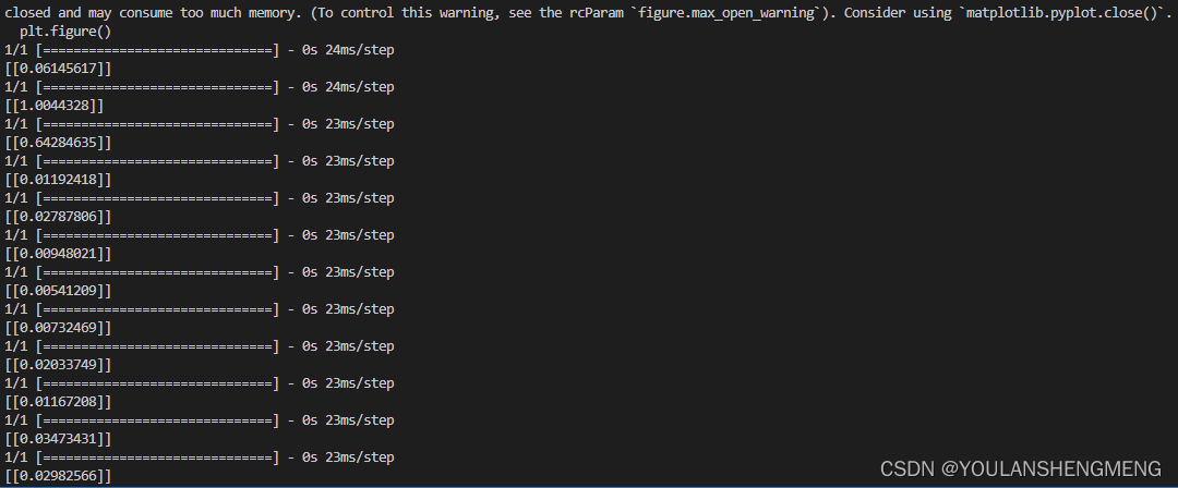
        plt.show()

测试结果显示：

五、使用孪生网络做指纹识别

参考链接： 指纹识别实战--基于TensorFlow实现-腾讯云开发者社区-腾讯云 (tencent.com)

1）孪生网络的检测原理

孪生神经网络英文简称为Siamese网络,它的主体结构是由一对共享相同权值的神经网络所组成的，通常被用于来计算数据之间的相似度，也正是因为具有相同的权值，因此才被称为“孪生”。值得注意的是，它并不是一个具体的神经网络模型，而只是一个架构，其中两边的输入网络可以被自定义设置为具体的CNN卷积神经网络或其它模型。

通常来说，输入到孪生神经网络里的一对数据最后都会被分别转换成一个向量的形式，之后根据这二者向量之间的差异来得到它们之间的相似度，例如常见的度量指标有欧氏距离和余弦距离等。整个网络的训练目标是让两个相似的输入距离尽可能的小，而让两个不同类别或差异较大的输入距离尽可能的大。以人脸识别为例，同一个人的脸被认为是相似输入，而不同人的人脸即被认为是不同输入，其示意图如图所示。

 2）数据集准备

2.1 数据下载

       将孪生神经网络应用到当前的指纹识别实战任务中去，即是将网络的输入数据替换成指纹图像。同一个人的指纹输入即为相似输入，对应的标签为1。不同人的指纹输入即为不同输入，标签为0。而该网络的设计目的便是让它可以根据输入的指纹图像来判断这对指纹是否属于同一个人，即达到指纹识别的目的。通常其中一个输入可被视为是保存在数据库里的指纹模板，另一个输入则是当前用户访问服务时被采集到的指纹数据，其模型示意图如图4所示。

所使用的指纹数据来自于中国科学院生物特征与安全研究中心里的指纹数据库，其数据下载网站为： http://biometrics.idealtest.org/findTotalDbByMode.do?mode=Fingerprint。如何下载可以参考原参考链接中的下载方法。

整个CASIA指纹数据集一共由5880张指纹组成，它们分别采自于不同的实验对象，其中针对每个实验对象的左、右食指和中指进行一共20次指纹图像的采集，即每个手指分别会被采集5次，图10展示了CASIA数据中的一个试验者被采集到的左、右食指和中指的指纹图像。

2.2 数据配准 

由于在CASIA指纹数据集中，采集到的指纹数据特征有可能各不相同，有些采集到的指纹特征甚至已经遭到破坏(如潮湿、刮伤等)，因此分析这种包含各种真实情况的指纹数据集会更加具有实际意义。而在利用孪生神经网络对不同人的指纹进行匹配之前，最重要的一步那便是指纹的对齐操作。

由于在指纹采集的过程中手指会产生旋转、偏移或错位，因此采集到的指纹图像其中很多都是无法正常对齐的，特征点无法直接进行匹配。所以需要先将数据配准。

单独两张图像的配准代码如下：

import cv2
import numpy as np
import os
import matplotlib.pyplot as plt

def alignImages(im1, im2):
    im1Gray = cv2.cvtColor(im1, cv2.COLOR_BGR2GRAY)   #将图片转换为灰度图
    im2Gray = cv2.cvtColor(im2, cv2.COLOR_BGR2GRAY)
    sift = cv2.xfeatures2d.SIFT_create()   #调用SIFT算法
    keypoints1, descriptors1 = sift.detectAndCompute(im1Gray, None)   #检测特征点和描述符
    keypoints2, descriptors2 = sift.detectAndCompute(im2Gray, None)
    
    matcher = cv2.BFMatcher()   #调用Brute Force匹配算法
    matches = matcher.match(descriptors1, descriptors2, None)   #对两张指纹图像进行匹配
    matches.sort(key=lambda x: x.distance, reverse=False)   #将匹配分数进行排序
    numGoodMatches = int(len(matches)*0.2)   #选取排序得分前20%的指纹
    
    matches = matches[:numGoodMatches]
    #绘制匹配点
    imMatches = cv2.drawMatches(im1, keypoints1, im2, keypoints2, matches, None)
    
    cv2.imwrite("matches.jpg", imMatches)   #保存匹配图像

    points1 = np.zeros((len(matches), 2), dtype=np.float32)
    points2 = np.zeros((len(matches), 2), dtype=np.float32)
    for i, match in enumerate(matches):   #提取匹配点的位置
        points1[i, :] = keypoints1[match.queryIdx].pt 
        points2[i, :] = keypoints2[match.trainIdx].pt  
    h, mask = cv2.findHomography(points1, points2, cv2.RANSAC)   #寻找仿射矩阵
    height, width, channels = im2.shape
    
    im1Reg = cv2.warpPerspective(im1, h, (width, height))   #对匹配图像进行对齐   
    return im1Reg, h

if __name__ == "__main__":

    refFilename = "0403_00032_0001_1_S.bmp"   
    imReference = cv2.imread(refFilename, cv2.IMREAD_COLOR)   #读取图像
    imFilename = "0403_00032_0002_2_S.bmp"
    im = cv2.imread(imFilename, cv2.IMREAD_COLOR)
    imReg, h = alignImages(im, imReference)   #对齐图像
    outFilename = "aligned.bmp"   #存储对齐图像的名称
    cv2.imwrite(outFilename, imReg)   #保存对齐图像
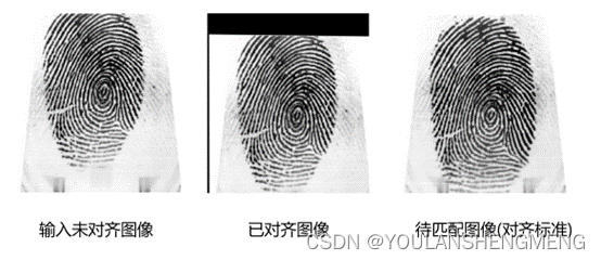
    print("Estimated homography : \n",  h)   #输出单适应矩阵

配准后 的结果示例如图所示：可以看出在对齐之前，输入的指纹图像与待匹配图像从位置上无法一一对应，而在对齐之后，以如图所示的指纹中间的螺旋纹为标准，可以看出两个指纹已成功完成对齐操作。但是很明显可以看出在执行SIFT算法之后，生成的对齐图像缺失了一部分图像信息，这部分信息是原图之前所没有的，在SIFT算法里会直接将它们填充成无关的背景色。

    之后将SIFT算法应用于CASIA数据集上，作为实战案例这里只选取了其中一小部分数据集进行指纹识别项目演示。以同一个人相同手指的第一张指纹图像作为对齐标准，剩下的四张指纹图像作为待对齐的图像。首先需要生成指定要求的对应文件路径，方便后续进行对齐并加载保存：

import cv2
import numpy as np
import os
import matplotlib.pyplot as plt

def alignImages(im1, im2):
    im1Gray = cv2.cvtColor(im1, cv2.COLOR_BGR2GRAY)   #将图片转换为灰度图
    im2Gray = cv2.cvtColor(im2, cv2.COLOR_BGR2GRAY)
    sift = cv2.xfeatures2d.SIFT_create()   #调用SIFT算法
    keypoints1, descriptors1 = sift.detectAndCompute(im1Gray, None)   #检测特征点和描述符
    keypoints2, descriptors2 = sift.detectAndCompute(im2Gray, None)
    
    matcher = cv2.BFMatcher()   #调用Brute Force匹配算法
    matches = matcher.match(descriptors1, descriptors2, None)   #对两张指纹图像进行匹配
    matches.sort(key=lambda x: x.distance, reverse=False)   #将匹配分数进行排序
    numGoodMatches = int(len(matches)*0.2)   #选取排序得分前20%的指纹
    
    matches = matches[:numGoodMatches]
    #绘制匹配点
    imMatches = cv2.drawMatches(im1, keypoints1, im2, keypoints2, matches, None)
    
    cv2.imwrite("matches.jpg", imMatches)   #保存匹配图像

    points1 = np.zeros((len(matches), 2), dtype=np.float32)
    points2 = np.zeros((len(matches), 2), dtype=np.float32)
    for i, match in enumerate(matches):   #提取匹配点的位置
        points1[i, :] = keypoints1[match.queryIdx].pt 
        points2[i, :] = keypoints2[match.trainIdx].pt  
    h, mask = cv2.findHomography(points1, points2, cv2.RANSAC)   #寻找仿射矩阵
    height, width, channels = im2.shape
    
    im1Reg = cv2.warpPerspective(im1, h, (width, height))   #对匹配图像进行对齐   
    return im1Reg, h

if __name__ == "__main__":

    #读取数据集路径
    dir_path = r'D:\Project_code\fingerPrint\CASIA_Fingerprint_Subject_Ageing\2013\uru4000\2' 
    folder_list = os.listdir(dir_path)   #查看该路径下文件夹信息
    #得到每个文件夹的具体路径
    imagePath_list = [os.path.join(dir_path, imageName) for imageName in folder_list] 
    imageAlignedPath = []
    for i in imagePath_list:
        firstIndex = 0
        imageName_list = os.listdir(i)   #遍历每个文件夹下的图片名称
        for j in range(len(imageName_list)):
            if j == firstIndex:           
                continue
            elif j%5==0:                 
                firstIndex+=5
            else:
                image1Path_list = [os.path.join(i, imageName_list[firstIndex])]  
                imageAlignedPath.append(image1Path_list)        
                image2Path_list = [os.path.join(i, imageName_list[j])]    
                #准备待对齐的指纹路径，格式为前面一张为指纹对齐参考图像，后一张为待对齐图像，不断循环
                imageAlignedPath.append(image2Path_list)

    #读取制作好的指纹图像文件路径，调用SIFT算法对它们进行一一匹配并保存至指定文件夹中：
    i = 0 
    name = 1
    while i < len(imageAlignedPath):
        reference = cv2.imread(imageAlignedPath[i][0], cv2.IMREAD_COLOR)   #读取指纹对齐参考图像  
        aligned = cv2.imread(imageAlignedPath[i+1][0], cv2.IMREAD_COLOR)   #读取待对齐的图像
        aligned_out, h = alignImages(reference, aligned)   #对齐图像
        reference_outName = imageAlignedPath[i][0][-23:-4]   #读取指纹对齐参考图像文件名
        aligned_outName = imageAlignedPath[i+1][0][-23:-4]   #读取指纹待对齐图像的文件名
        #参考图像和对齐图像的存储路径
        save_path1 = r'D:\Project_code\fingerPrint\dataset\Genuine\(6)unaligned_souce\reference'
        save_path2 = r'D:\Project_code\fingerPrint\dataset\Genuine\(6)unaligned_souce\aligned'
        print("Reference image : ", reference_outName)
        print("Saving aligned image : ", aligned_outName) 
        reference_savePath = save_path1 + "\\" + str(name) +'.jpg'
        aligned_savePath = save_path2 + "\\" + str(name) +'.jpg'
        cv2.imwrite(reference_savePath,reference)   #存储指纹对齐参考图像
        cv2.imwrite(aligned_savePath,aligned_out)   #存储已对齐的指纹图像
        i+=2
        name+=1 

输出结果为：

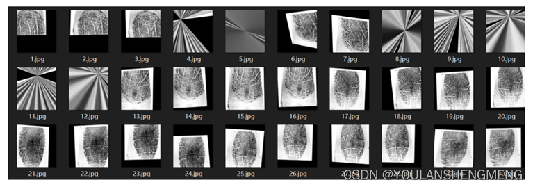
有部分数据，会因为特征点的数目过少，导致配准失败，在训练前需要将配准失败的数据删除。最终待训练的数据结果如图所示：

3）模型搭建及训练

        在对指纹数据集进行对齐和一定的预处理操作之后，下一步便是将这些成对的指纹图像送入到孪生神经网络中以便于完成指纹识别任务的训练，匹配指纹图像和指纹模板图像各自选取278张，其中139张为同一个人相同手指的指纹，139张为不同人相同手指的指纹。所以这个后139张图像的标签为0.

下面的代码包含了对数据集的数据转换、网络搭建、损失的定义、网络的训练、网络模型的保存。

import tensorflow as tf
from tensorflow import keras 
import cv2
import os
import matplotlib.pyplot as plt
import numpy as np
from tensorflow.keras import backend as K
from tensorflow.keras.preprocessing import image

#训练数据的路径，数据是经过配准的，是使用配准后的图像进行训练的
Train_referencePath = r'D:\Project_code\fingerPrint\dataset\Genuine\(2)Reference'
Train_alignedPath = r'D:\Project_code\fingerPrint\dataset\Genuine\(2)Aligned'

#读取路径下的图像数据，并将它们储存至列表当中，方便模型后续处理：
referenceTrain = []
alignedTrain = []
Train_sourceImageList = os.listdir(Train_referencePath)
Train_sourceImageList.sort(key=lambda x:int(x[:-4]))
Train_alignedImageList = os.listdir(Train_alignedPath)
Train_alignedImageList.sort(key=lambda x:int(x[:-4]))
for i in Train_sourceImageList:
    imagePath = os.path.join(Train_referencePath,i)   #读取reference图像路径
    referenceImage = image.load_img(imagePath)   #加载图像成jpg格式
    img_array = image.img_to_array(referenceImage)   #转换成array格式
    referenceTrain.append(img_array)   #保存至列表
for i in Train_alignedImageList:
    imagePath = os.path.join(Train_alignedPath,i)
    alignedImage = image.load_img(imagePath)
    img_array = image.img_to_array(alignedImage)
    alignedTrain.append(img_array)

#将列表形式转换为numpy数组：
print("Original type:%s"%type(referenceTrain))
referenceTrain = np.array(referenceTrain)   #转换图像类型
alignedTrain = np.array(alignedTrain)
print("Converted type:%s"%type(referenceTrain))  

#数据的归一化处理
referenceTrain = referenceTrain.astype('float32')/255   #图像归一化
alignedTrain = alignedTrain.astype('float32')/255
print(alignedTrain[-1].shape)   #查看图像尺寸

#标签的制作 匹配指纹图像和指纹模板图像各自选取278张，其中139张为同一个人相同手指的指纹，139张为不同人相同手指的指纹
labels = [1]*139 + [0]*139   #制作图像标签
labels = np.array(labels).astype('float32')   #标签类型转换
print(type(labels))

#定义以欧氏距离为基础的输入图像对的距离衡量函数，对抗损失函数以及准确率指标计算函数:
def euclidean_distance(vects):   #向量欧式距离计算
    x, y = vects
    sum_square = K.sum(K.square(x - y), axis=1, keepdims=True)
    return K.sqrt(K.maximum(sum_square, K.epsilon()))  

def eucl_dist_output_shape(shapes):   #结果输出维度
    shape1, shape2 = shapes
    return (shape1[0], 1)

def contrastive_loss(y_true, y_pred):   #对抗损失函数
    margin = 1
    sqaure_pred = K.square(y_pred)
    margin_square = K.square(K.maximum(margin - y_pred, 0))
    return K.mean(y_true * sqaure_pred + (1 - y_true) * margin_square)

def accuracy(y_true, y_pred):   #模型训练评判指标
    return K.mean(K.equal(y_true, K.cast(y_pred <0.5, y_true.dtype)))


#定义孪生神经网络的模型架构   其中卷积层里的dilation_rate表示的是空洞卷积的扩张率，经过不断的前向传播，最后模型会输出一个向量值用来衡量图像间的距离和相似度：
def MDCNN_network(input_shape):   #模型搭建
    input = keras.layers.Input(shape = input_shape)
    x = keras.layers.Conv2D(filters=2,kernel_size=3,input_shape=(356,328,3))(input)
    x = keras.activations.selu(x)
    x1 = keras.layers.Conv2D(filters=4,kernel_size=3,strides=1,padding='same')(x)
    x1 = keras.activations.selu(x1)
    x2 = keras.layers.Conv2D(filters=4,kernel_size=3,strides=1,dilation_rate=(2,2),padding='same')(x)
    x2 = keras.activations.selu(x2)
    x3 = keras.layers.Conv2D(filters=4,kernel_size=3,strides=1,dilation_rate=(3,3),padding='same')(x)
    x3 = keras.activations.selu(x3)
    x = keras.layers.Add()([x1,x2,x3])
    x = keras.layers.Conv2D(filters=8,kernel_size=3)(x)
    x = keras.activations.selu(x)
    x1 = keras.layers.Conv2D(filters=16,kernel_size=3,strides=2)(x)
    x1 = keras.activations.selu(x1)
    x2 = keras.layers.Conv2D(filters=16,kernel_size=3,strides=2)(x)
    x2 = keras.activations.selu(x2)
    x3 = keras.layers.Conv2D(filters=16,kernel_size=3,strides=2)(x)
    x3 = keras.activations.selu(x3)
    x = keras.layers.Add()([x1,x2,x3])
    x = keras.layers.Conv2D(filters=32,kernel_size=3)(x)
    x = keras.activations.selu(x)
    x = keras.layers.Conv2D(filters=64,kernel_size=3,strides=2)(x)
    x = keras.activations.selu(x)
    x = keras.layers.Flatten()(x)
    x = keras.layers.Dense(10)(x)
    return keras.models.Model(input, x)

#利用先前定义过的距离函数，将模型的输出转换成欧式距离上的衡量，并将它拼接至搭建的模型上：
base_network = MDCNN_network(referenceTrain[0].shape)
input_a = keras.Input(shape=referenceTrain[0].shape)
input_b = keras.Input(shape=alignedTrain[0].shape)
processed_a = base_network(input_a)   #模型一路输入
processed_b = base_network(input_b)   #模型另一路输入
distance = keras.layers.Lambda(euclidean_distance,output_shape=eucl_dist_output_shape)([processed_a, processed_b])
model = keras.models.Model([input_a, input_b], distance)   #模型拼接

#配置模型的损失函数、优化器、评价指标等相关训练参数：
model.compile(loss=contrastive_loss,optimizer='adam',metrics=[accuracy])

#对模型进行训练：epochs=10可以设置训练的次数
history=model.fit([referenceTrain, alignedTrain],labels,batch_size=1,epochs=10,verbose=1)

model.save("trainmodel.h5")

定义孪生神经网络的模型架构，这里采用多尺度空洞卷积组合所构成的神经网络，该模型已被相关文献证明是一个能够提取不同尺度的指纹细节点特征的匹配网络结构。其中模型示意图如图所示： 

4）模型的推理

import tensorflow as tf
from tensorflow import keras 
import cv2
import os
import matplotlib.pyplot as plt
import numpy as np
from tensorflow.keras import backend as K
from tensorflow.keras.preprocessing import image

#定义以欧氏距离为基础的输入图像对的距离衡量函数，对抗损失函数以及准确率指标计算函数:
def euclidean_distance(vects):   #向量欧式距离计算
    x, y = vects
    sum_square = K.sum(K.square(x - y), axis=1, keepdims=True)
    return K.sqrt(K.maximum(sum_square, K.epsilon()))  

def eucl_dist_output_shape(shapes):   #结果输出维度
    shape1, shape2 = shapes
    return (shape1[0], 1)

def contrastive_loss(y_true, y_pred):   #对抗损失函数
    margin = 1
    sqaure_pred = K.square(y_pred)
    margin_square = K.square(K.maximum(margin - y_pred, 0))
    return K.mean(y_true * sqaure_pred + (1 - y_true) * margin_square)

def accuracy(y_true, y_pred):   #模型训练评判指标
    return K.mean(K.equal(y_true, K.cast(y_pred <0.5, y_true.dtype)))

model = keras.models.load_model("../trainmodel.h5",custom_objects={'contrastive_loss':contrastive_loss,'accuracy':accuracy})  


def testImage_preprocessing(image_path):   #测试图像预处理函数
    testImage = image.load_img(image_path)   #图像加载
    plt.imshow(testImage)
    plt.show()
    testImage = image.img_to_array(testImage).astype('float32')/255
    testImage = np.expand_dims(testImage,axis=0)   #图像维度增添以满足模型输入要求
    return testImage


# Train_referencePath = '..CASIA_code/data/pdf/'
# Train_alignedPath = '..CASIA_code/data/image/'


same_path_1 = '/home/sim_code/CASIA_code/data/pdf/0.bmp'
same_path_2 = '/home/sim_code/CASIA_code/data/image/0.bmp'
different_path_1 = '/home/sim_code/CASIA_code/data/pdf/80.bmp'
different_path_2 = '/home/sim_code/CASIA_code/data/image/80.bmp'
same_testImage_1 = testImage_preprocessing(same_path_1)
same_testImage_2 = testImage_preprocessing(same_path_2)
different_testImage_1 = testImage_preprocessing(different_path_1)
different_testImage_2 = testImage_preprocessing(different_path_2)

sameScore = model.predict([same_testImage_1,same_testImage_2]) #相同指纹距离预测
differentScore = model.predict([different_testImage_1,different_testImage_2]) #不同指纹距离预测

print("The distance of same fingerprint:%f"%sameScore[0][0])
print("The distance of different fingerprint:%f"%differentScore[0][0])

推理的结果为：

六、用孪生网络做人脸相似性识别

参考博文： 基于改进孪生网络的人脸识别方法（讲解+代码V1.0）-CSDN博客

代码下载地址：GitHub - damoshishen/FR_twin_network: In this paper, a small sample face recognition algorithm and system design based on improved twin network are reproduced.基础环境：tensorflow+keras