目录
3、创建配置类,将LSTM的各个超参数声明为变量,便于后续使用
一、数据集
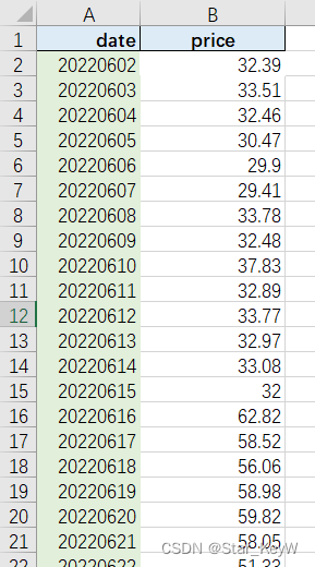
自建数据集--【load.xlsx】。包含2列:
- date列(时间列,记录2022年6月2日起始至2023年12月31日为止,日度数据)
- price列(价格列,记录日度数据对应的某品牌衣服的价格,浮点数)
二、任务目标
实现基于时间序列的单特征价格预测
三、代码实现
1、从本地路径中读取数据文件
- read_excel函数读取Excel文件(read_csv用来读取csv文件),并设置为DataFrame对象
- index_col='date'将'date'列设置为DataFrame的索引
- .values属性获取price列的值,pandas会将对应数据转换为NumPy数组
# 字符串前的r表示一个"原始字符串",raw string
# 文件路径中包含多个反斜杠。如果我们不使用原始字符串(即不使用r前缀),那么Python会尝试解析\U、\N等作为转义序列,这会导致错误
data = pd.read_excel(r'E:\load.xlsx', index_col='date')
# print(data)
prices = data['price'].values
# print(prices)打印data:

打印prices:

2、数据归一化
- 归一化:将原始数据的大小转化为[0,1]之间,采用最大-最小值归一化
- 数值过大,造成神经网络计算缓慢
- 在多特征任务中,存在多个特征属性,但神经网络会认为数值越小的,影响越小。所以可能关键属性A的值很小,不重要属性B的值却很大,造成神经网络的混淆
- scikit-learn的转换器通常期望输入是二维的,其中每一行代表一个样本,每一列代表一个特征
- prices.reshape(-1, 1) 用于确保 prices 是一个二维数组,即使它只有一个特征列
- -1的意思是让 NumPy 自动计算该轴上的元素数量,以保持原始数据的元素总数不变
- fit方法计算了数据中每个特征的最小值和最大值,这些值将被用于缩放
- transform方法使用这些统计信息来实际缩放数据,将其转换到 [0, 1] 范围内
scaler = MinMaxScaler(feature_range=(0, 1))
scaled_prices = scaler.fit_transform(prices.reshape(-1, 1)) # 二维数组
# print(scaled_prices)打印归一化后的价格数据:

3、创建配置类,将LSTM的各个超参数声明为变量,便于后续使用
- timestep:时间步长,滑动窗口大小
- feature_size:每个步长对应的特征数量,这里只使用1维,即每天的价格数据
- batch_size:批次大小,即一次性送入多少个数据(一时间步长为单位)进行训练
- output_size:单输出任务,输出层为1,预测未来1天的价格
- hidden_size:隐藏层大小,即神经元个数
- num_layers:神经网络的层数
- learning_rate:学习率
- epochs:迭代轮数,即总共要让神经网络训练多少轮,全部数据训练一遍成为一轮
- best_loss:记录损失
class Config():
    timestep = 7  # 时间步长,滑动窗口大小
    feature_size = 1 # 每个步长对应的特征数量,这里只使用1维,每天的价格数据
    batch_size = 1 # 批次大小
    output_size = 1 # 单输出任务,输出层为1,预测未来1天的价格
    hidden_size = 128 # 隐藏层大小
    num_layers = 1 # lstm的层数
    learning_rate = 0.0001 # 学习率
    epochs = 500 # 迭代轮数
    model_name = 'lstm' # 模型名
    best_loss = 0  # 记录损失
config = Config()
4、创建时间序列数据
- 通过滑动窗口移动获取数据,时间步内数据作为特征数据,时间步外1个数据作为标签数据
- 通过序列的切片实现特征和标签的划分
- 通过np.array将数据转化为NumPy数组

# 创建时间序列数据
X, y = [], []
for i in range(len(scaled_prices) - config.timestep):
    # 从当前索引i开始,取sequence_length个连续的价格数据点,并将其作为特征添加到列表 X 中。
    X.append(scaled_prices[i: i + config.timestep])
    # 将紧接着这sequence_length个时间点的下一个价格数据点作为目标添加到列表y中。
    y.append(scaled_prices[i + config.timestep])
X = np.array(X)
y = np.array(y)打印特征数据:

打印标签数据:

5、划分数据集
- 按照9:1的比例划分训练集和测试集
- 因为时间序列数据具有时序性,用过去时间数据预测新时间数据,要保证时间有序
- 测试数据为时间序列的末尾数据
# 确定测试集的大小
test_size = int(len(scaled_prices) * 0.1)

# 为了确保训练集和测试集的划分不会破坏时间序列的连续性,我们需要从时间序列的开头开始划分训练集。
X_train = X[:-test_size]
y_train = y[:-test_size]
X_test = X[-test_size:]
y_test = y[-test_size:]
6、将数据转化为PyTorch张量
- PyTorch使用张量作为其基本数据结构,类似于NumPy中的ndarray,但张量可以在GPU上进行加速计算
- 神经网络通常需要单精度浮点数进行计算
X_train_tensor = torch.tensor(X_train, dtype=torch.float32)
y_train_tensor = torch.tensor(y_train, dtype=torch.float32)
X_test_tensor = torch.tensor(X_test, dtype=torch.float32)
y_test_tensor = torch.tensor(y_test, dtype=torch.float32)打印X_train_tensor:

打印y_train_tensor:

7、将数据加载成迭代器
- 使用TensorDataset从PyTorch的torch.utils.data模块创建训练数据集和测试数据集。这些数据集对象可以方便地与PyTorch的数据加载器(如DataLoader)一起使用,以在模型训练和评估过程中提供批量数据
- 当你使用DataLoader来加载训练和测试数据集时,它会自动将数据分批处理成符合LSTM网络的输入格式:(batch_size, sequence_length, feature_size)
- 这里的batch_size由config.batch_size指定
- sequence_length是config.timestep
- feature_size在这个例子中是1,因为只有一个特征
- shuffle=False:指定是否在每个训练时开始时随机打乱数据。因为时间序列数据,要保证数据的有序性
# 形成训练数据集
train_data = TensorDataset(X_train_tensor, y_train_tensor)
test_data = TensorDataset(X_test_tensor, y_test_tensor)

# 将数据加载成迭代器
train_loader = torch.utils.data.DataLoader(train_data, batch_size=config.batch_size, shuffle=False)
test_loader = torch.utils.data.DataLoader(test_data, batch_size=config.batch_size, shuffle=False)打印迭代器:

8、定义LSTM网络
- torch.nn.Module类是所有神经网络模块的基类
- 参数batch_first=True意味着输入张量的形状应该是[batch_size, sequence_length, input_size]
- 在PyTorch中,全连接层被命名为 fc(代表“fully connected”)
- 全连接层通常是通过 nn.Linear 类来实现的
- 在神经网络的定义中创建一个nn.Linear实例并将其赋值给一个成员变量(如 self.fc)时,实际上是在网络中嵌入了一个全连接层
- 这个层会在forward方法中被调用,对LSTM的输出进行线性变换
class LSTM(nn.Module):
    # __init__方法用于初始化模型的各种层和参数
    def __init__(self, feature_size, hidden_size, num_layers, output_size):
        super(LSTM, self).__init__()
        self.hidden_size = hidden_size
        self.num_layers = num_layers
        # 参数batch_first=True意味着输入张量的形状应该是[batch_size, sequence_length, input_size]
        self.lstm = nn.LSTM(feature_size, hidden_size, num_layers, batch_first=True)
        # input_size 是全连接层的输入特征数,output_size 是输出特征数
        self.fc = nn.Linear(hidden_size, output_size)

    # forward方法定义了输入数据通过模型各层的前向传播过程。
    # 模型的forward方法被自动调用,并且X_train_batch作为参数传递给这个方法。
    def forward(self, x, hidden=None):
        # 获取输入数据x的第一维度的大小,即批量大小(batch size)
        # x的形状通常是 (batch_size, sequence_length, feature_size)
        batch_size = x.shape[0]

        # 初始化隐藏层状态
        # 如果隐藏状态hidden没有被提供(即为 None),则使用全零张量来初始化LSTM的隐藏状态h_0和细胞状态c_0
        if hidden is None:
            h_0 = x.data.new(self.num_layers, batch_size, self.hidden_size).fill_(0).float()
            c_0 = x.data.new(self.num_layers, batch_size, self.hidden_size).fill_(0).float()
        else:
            h_0, c_0 = hidden

        # LSTM运算
        # 将输入数据 x 和初始化的隐藏状态 (h_0, c_0) 传递给LSTM层,进行前向计算。
        # LSTM层的输出包含两部分:输出序列lstm_output 和 最终的隐藏状态
        # LSTM层在其内部单元中使用了sigmoid和tanh激活函数来处理输入和循环连接
        # self.lstm(x, (h_0, c_0))时,LSTM层内部的计算已经包括了激活函数的应用
        lstm_output, (h_0, c_0) = self.lstm(x, (h_0, c_0))

        # 取最后一个时间步的输出
        # lstm_output 的形状是 (batch_size, sequence_length, hidden_size)
        # ::第一个维度(批量维度)取全部。
        # -1:第二个维度(序列长度维度)取最后一个元素。在 Python 中,-1 索引表示从末尾开始计数的第一个元素。
        # ::第三个维度(隐藏层大小维度)取全部。
        final_output = lstm_output[:, -1, :]

        # 全连接层
        # 回归任务的目标是预测一个连续值,而不是进行分类,因此输出层应该能够直接产生实数范围的输出
        # 在PyTorch中,如果你不指定激活函数,nn.Linear层默认就是线性的,即它不会对其输出应用任何非线性函数
        output = self.fc(final_output)

        return output
9、创建LSTM实例
- model.parameters()是一个包含模型所有可训练参数的迭代器
- Adam是一种自适应学习率的优化算法,它结合了Momentum和RMSprop的思想,通常在很多任务上表现良好
# 创建了一个LSTM模型的实例
model = LSTM(config.feature_size, config.hidden_size, config.num_layers, config.output_size)
# 损失函数
loss_function = nn.MSELoss()
# 创建一个Adam优化器的实例,用于在训练过程中更新模型的权重
optimizer = torch.optim.Adam(model.parameters(), lr=config.learning_rate)
10、训练模型
11、模型验证
- train()函数是torch.nn.Module类的一个方法
- eval()验证模型性能
# 训练模型
for epoch in range(config.epochs):
    # train()函数是torch.nn.Module类的一个方法
    model.train()
    train_loss_sum = 0.0
    # 形成进度条
    train_bar = tqdm(train_loader)
    for data in train_bar:
        X_train_batch, y_train_batch = data
        # 这行代码清除了之前优化步骤中累积的所有梯度。由于PyTorch在反向传播时默认会累积梯度,所以在每个新的优化步骤开始之前,需要手动清除它们。
        optimizer.zero_grad()
        # 通过模型进行前向传播以获取预测值(y_train_pred)
        y_train_pred = model(X_train_batch)
        # 预测值和真实值(y_train_batch)之间的损失。
        loss = loss_function(y_train_pred, y_train_batch.view(-1))
        # 进行反向传播。它计算损失相对于模型参数的梯度,这些梯度之后将被用于更新模型的权重。
        loss.backward()
        # 根据之前计算的梯度来更新模型的权重。具体来说,它使用之前定义的Adam优化器来调整模型的参数以最小化损失。
        optimizer.step()
        train_bar.desc = "train epoch[{} / {}] loss:{:.3f}".format(epoch + 1, config.epochs, loss)

    # 当你想要使用已经训练好的模型来预测新的、未见过的数据时,你需要确保模型处于评估模式
    # 在每个epoch结束后,,模型验证
    # model.eval()会改变模型中特定层的行为,如Dropout和BatchNorm层,使它们在推理时保持固定
    # 在训练模式中,这些层可能会引入随机性或根据训练数据的统计信息进行归一化;而在评估模式中,它们会保持确定性行为,以确保输出的一致性
    model.eval()
    test_loss_sum = 0.0
    y_test_preds = [] # 初始化一个空列表来保存所有预测结果
    y_test_true = []  # 初始化一个空列表来保存所有真实值
    test_bar = tqdm(test_loader)
    # 使用了torch.no_grad()上下文管理器来确保在验证过程中不计算梯度,因为不需要更新模型的权重,从而节省内存
    with torch.no_grad():
        for data in test_bar:
            X_test_batch, y_test_batch = data
            # 将测试数据X_test传递给模型,并接收模型的预测输出
            # 由于梯度计算被禁用,这个前向传播过程会更快,并且不会消耗额外的资源来存储梯度信息。
            y_test_pred = model(X_test_batch) # 获取当前批次的预测结果
            # 通常用于累积测试损失(test loss)
            test_loss = loss_function(y_test_pred, y_test_batch.view(-1))
            # test_loss.item()将PyTorch张量(tensor)中的单个值(在这种情况下是一个标量,即损失值)转换为Python数字(通常是浮点数)
            # 在评估模型性能时,能够计算整个测试集的平均损失,而不仅仅是单个批次或样本的损失
            # 通过累积所有批次或样本的损失,并在最后除以总的批次数或样本数,你可以得到一个更准确的模型性能估计
            test_loss_sum += test_loss.item()  # 累加损失
            y_test_preds.append(y_test_pred.detach().numpy())  # 将预测结果追加到列表中
            y_test_true.append(y_test_batch.detach().numpy())  # 将真实值追加到列表中
    test_loss_avg = test_loss_sum / len(test_loader)  # 计算平均测试损失
    y_test_preds= np.concatenate(y_test_preds, axis=0)  # 将所有批次的预测结果连接成一个数组
    y_test_true = np.concatenate(y_test_true, axis=0)  # 将所有批次的真实值连接成一个数组

    # 反归一化预测值和真实值
    # scaler.inverse_transform(...):使用之前拟合的 MinMaxScaler 将缩放后的预测值转换回其原始尺度
    # 以便在原始尺度上评估模型性能
    y_test_preds_unnormalized = scaler.inverse_transform(y_test_preds)
    y_test_true_unnormalized = scaler.inverse_transform(y_test_true.reshape(-1, 1))

    if test_loss_avg < config.best_loss:
        config.best_loss = test_loss_avg
print("训练结束")
12、绘制图像
# 绘制真实值和预测值的对比图
# 创建一个新的图形窗口,并设置其大小为宽10英寸、高5英寸。
plt.figure(figsize=(10, 5))
# 绘制真实值(y_test)的折线图,并为其添加标签 "True Values"。
plt.plot(y_test_true_unnormalized, label='True Values')
# 绘制预测值(predicted)的折线图。这条线被标记为 "Predicted Values"。
plt.plot(y_test_preds_unnormalized, label='Predictions')
plt.title('Comparison of True Values and Predictions')
plt.xlabel('Time Steps')
plt.ylabel('Prices')
plt.legend()
plt.show()
13、完整版
import pandas as pd
import numpy as np
import torch
from sklearn.preprocessing import MinMaxScaler
from torch import nn
from torch.utils.data import TensorDataset
from tqdm import tqdm
import matplotlib.pyplot as plt

class Config():
    timestep = 1  # 时间步长,滑动窗口大小
    feature_size = 1 # 每个步长对应的特征数量,这里只使用1维,每天的价格数据
    batch_size = 1 # 批次大小
    output_size = 1 # 单输出任务,输出层为1
    hidden_size = 128 # 隐藏层大小
    num_layers = 1 # bilstm的层数
    learning_rate = 0.0001 # 学习率
    epochs = 500 # 迭代轮数
    model_name = 'lstm' # 模型名
    best_loss = 0  # 记录损失
config = Config()

qy_data = pd.read_excel(r'C:\Users\Desktop\load.xlsx', index_col='date')
prices = qy_data['price'].values

scaler = MinMaxScaler()
scaled_prices = scaler.fit_transform(prices.reshape(-1, 1))

# 创建时间序列数据
X, y = [], []
for i in range(len(scaled_prices) - config.timestep):
    X.append(scaled_prices[i: i + config.timestep])
    y.append(scaled_prices[i + config.timestep])
X = np.array(X)
y = np.array(y)

# 确定测试集的大小
test_size = int(len(scaled_prices) * 0.1)

# 创建训练和测试数据
X_train, y_train = [], []
X_test, y_test = [], []

# 构建训练数据
for i in range(len(scaled_prices) - config.timestep - test_size):
    X_train.append(scaled_prices[i:i + config.timestep])
    y_train.append(scaled_prices[i + config.timestep])

# 构建测试数据(取时间序列末尾的数据)
for i in range(len(scaled_prices) - config.timestep - test_size, len(scaled_prices) - config.timestep):
    X_test.append(scaled_prices[i:i + config.timestep])
    y_test.append(scaled_prices[i + config.timestep])

# 将列表转换为NumPy数组
X_train = np.array(X_train)
y_train = np.array(y_train)
X_test = np.array(X_test)
y_test = np.array(y_test)

# 将数据转换为PyTorch张量
X_train_tensor = torch.tensor(X_train, dtype=torch.float32)
y_train_tensor = torch.tensor(y_train, dtype=torch.float32)
X_test_tensor = torch.tensor(X_test, dtype=torch.float32)
y_test_tensor = torch.tensor(y_test, dtype=torch.float32)

# 形成训练数据集
train_data = TensorDataset(X_train_tensor, y_train_tensor)
test_data = TensorDataset(X_test_tensor, y_test_tensor)

# 将数据加载成迭代器
train_loader = torch.utils.data.DataLoader(train_data, batch_size=config.batch_size, shuffle=False)
test_loader = torch.utils.data.DataLoader(test_data, batch_size=config.batch_size, shuffle=False)

# 定义LSTM网络
class LSTM(nn.Module):
    # __init__方法用于初始化模型的各种层和参数
    def __init__(self, feature_size, hidden_size, num_layers, output_size):
        super(LSTM, self).__init__()
        self.hidden_size = hidden_size
        self.num_layers = num_layers
        self.lstm = nn.LSTM(feature_size, hidden_size, num_layers, batch_first=True)
        self.fc = nn.Linear(hidden_size, output_size)

    # forward方法定义了输入数据通过模型各层的前向传播过程。
    # 模型的forward方法被自动调用,并且X_train_batch作为参数传递给这个方法。
    def forward(self, x, hidden=None):
        batch_size = x.shape[0]

        if hidden is None:
            h_0 = x.data.new(self.num_layers, batch_size, self.hidden_size).fill_(0).float()
            c_0 = x.data.new(self.num_layers, batch_size, self.hidden_size).fill_(0).float()
        else:
            h_0, c_0 = hidden

        lstm_output, (h_0, c_0) = self.lstm(x, (h_0, c_0))

        lstm_output = self.dropout(lstm_output)

        final_output = lstm_output[:, -1, :]

        output = self.fc(final_output)

        return output


# 这行代码创建了一个LSTM模型的实例
model = LSTM(config.feature_size, config.hidden_size, config.num_layers, config.output_size, config.dropout)
loss_function = nn.MSELoss()
optimizer = torch.optim.Adam(model.parameters(), lr=config.learning_rate)

# 训练模型
for epoch in range(config.epochs):
    model.train()
    train_loss_sum = 0.0
    # 形成进度条
    train_bar = tqdm(train_loader)
    for data in train_bar:
        X_train_batch, y_train_batch = data
        optimizer.zero_grad()
        y_train_pred = model(X_train_batch)
        loss = loss_function(y_train_pred, y_train_batch.view(-1))
        loss.backward()
        optimizer.step()
        train_bar.desc = "train epoch[{} / {}] loss:{:.3f}".format(epoch + 1, config.epochs, loss)

    model.eval()
    test_loss_sum = 0.0
    y_test_preds = [] # 初始化一个空列表来保存所有预测结果
    y_test_true = []  # 初始化一个空列表来保存所有真实值
    test_bar = tqdm(test_loader)
    with torch.no_grad():
        for data in test_bar:
            X_test_batch, y_test_batch = data
            y_test_pred = model(X_test_batch) # 获取当前批次的预测结果
            test_loss = loss_function(y_test_pred, y_test_batch.view(-1))
            test_loss_sum += test_loss.item()  # 累加损失
            y_test_preds.append(y_test_pred.detach().numpy())  # 将预测结果追加到列表中
            y_test_true.append(y_test_batch.detach().numpy())  # 将真实值追加到列表中
    test_loss_avg = test_loss_sum / len(test_loader)  # 计算平均测试损失
    y_test_preds= np.concatenate(y_test_preds, axis=0)  # 将所有批次的预测结果连接成一个数组
    y_test_true = np.concatenate(y_test_true, axis=0)  # 将所有批次的真实值连接成一个数组

    # 反归一化预测值和真实值
    # scaler.inverse_transform(...):使用之前拟合的 MinMaxScaler 将缩放后的预测值转换回其原始尺度。
    # 以便在原始尺度上评估模型性能
    y_test_preds_unnormalized = scaler.inverse_transform(y_test_preds)
    y_test_true_unnormalized = scaler.inverse_transform(y_test_true.reshape(-1, 1))


    if test_loss_avg < config.best_loss:
        config.best_loss = test_loss_avg
        torch.save(model.state_dict(), config.save_path)
print("训练结束")

plt.figure(figsize=(10, 5))
plt.plot(y_test_true_unnormalized, label='True Values')
plt.plot(y_test_preds_unnormalized, label='Predictions')
plt.title('Comparison of True Values and Predictions')
plt.xlabel('Time Steps')
plt.ylabel('Prices')
plt.legend()
plt.show()


